What makes a transformer use both of its layers? Circuit formation in Dyck-(k, m)
Introduction
Mechanistic interpretability has assembled detailed, causal accounts of specialized attention circuits in trained transformers. The cleanest is the induction head first studied by Olsson et al. (2022) in In-context Learning and Induction Heads in the Transformer Circuits Thread — a two-layer circuit that completes [A][B] … [A] → [B] by attending back to the token that followed the previous occurrence of the current token. Induction heads are an unusually good object of study: they are reliably present in small attention-only models, and their appearance during training is marked by a visible phase change in the loss.
Most such accounts describe circuits in models that have already been trained. I wanted instead to watch a circuit form — to follow an identifiable head through training with every head, activation, and checkpoint available to inspect. That resolution rules out natural language: at the scales where language is learnable, a fully instrumented run from scratch is far beyond a modest compute and memory budget. To study circuit formation at all, the task has to be synthetic and small.
The most naive synthetic task is the induction task itself: one generates sequences of repeated random tokens and trains the model on next-token prediction. Unlike in natural language, the model finds a first-layer shortcut and never builds the two-layer composition that defines a genuine induction circuit. This is because in this task, the only structure to learn is the repetition within a sequence, which can be done in a single layer. In order for more complex heads to develop, the language of the task has to carry more structure than the shortcut can capture, or the model will simply take the shortcut.
The Dyck-$(k, m)$ language consists of balanced bracket sequences over $k$ types with nesting depth at most $m$ and is about the simplest context-free grammar that still has real structure. It separates two computational sub-tasks: depth tracking, a scalar running count, and type matching, a non-local lookup of the most recent unmatched OPEN. At $k = 1$ only depth tracking is non-trivial; at $k \geq 2$ both are required.
In this post I report what two-layer attention-only transformers actually learn for $k \in {1, 2, 3}$, where $k$ is used to control the structural complexity of the task. For Dyck-1 I find a two-head model reaches the entropy floor of the task without forming any induction-shaped circuitry at all. Layer 1 is inert, and strongly negative layer-0 copying scores reveal a “bracket-flipping” shortcut. This is the same single-layer escape the repeated-token task fell into. For Dyck-2 and Dyck-3 ($k\geq 2$) the type matching required forces the formation of a two-stage factored circuit. In this circuit layer 0 constructs a linear representation of bracket depth, demonstrated by the first principal component of the residual-stream correlating with ground-truth depth at $r = 0.75$, and layer 1 performs type-aware matching. Activation patching confirms this factorization causally and identifies the single causally dominant readout head as the head containing the lowest type-match score in its layer but with an OV circuit implementing the OPEN→CLOSE flip the task needs. This head would not have been flagged by attention-pattern analysis alone — it required looking at both the QK and OV circuits. Overall, I found that width controls factorization, not capability: a two-head model eventually solves Dyck-2 too, but via a qualitatively different, more entangled two-pathway circuit.
Code and executed notebooks: interp-repo.
Related work Dyck languages are a standard testbed for sequence models. Hewitt et al. (2020) introduced the Dyck-$(k, m)$ family and proved that RNNs can generate it with memory $O(m \log k)$ — the construction and bounded-depth setup this post borrows. For transformers, Yao et al. (2021) give a two-layer self-attention construction for bounded Dyck, with essentially the depth-plus-type-matching decomposition observed empirically here; Ebrahimi et al. (2020) study how self-attention processes Dyck-$n$; Liu et al. (2022) characterize shortcut solutions to automata-like tasks; and Wen et al. (2023) demonstrate solution multiplicity and the unreliability of attention-pattern analysis on bounded Dyck — conclusions the patching results and width comparison below independently corroborate at small scale. These experiments were run independently as a from-scratch exercise, and I have not systematically audited the overlap with prior results; they are presented as a self-contained empirical study rather than a claim of novelty.
Setup
Following Yao et al. (2021), I fix a vocabulary of $k$ bracket types, $\Sigma = \bigcup_{i \in [k]} {\,\langle_i,\ \rangle_i\,}$, where $\langle_i$ and $\rangle_i$ are the OPEN and CLOSE brackets of type $i$. $\mathsf{Dyck}_{k}$ is defined as the language of well-nested bracket strings, generated from the start symbol $X$ by the context-free grammar
\[X \;\to\; \varepsilon \;\;\big|\;\; \langle_i\, X\, \rangle_i\, X \qquad (i \in [k]),\]with $\varepsilon$ the empty string. The single recursive production $\langle_i X \rangle_i X$ is what forces every CLOSE to match the most recent unclosed OPEN of the same type — the defining constraint of the language. Reading a string left to right, the unmatched OPENs form a stack: an OPEN pushes its type, a CLOSE pops and must agree with the top. The depth at position $i$ is the stack height, equivalently the running excess of OPENs over CLOSEs,
\[d(w_{1:i}) = \mathsf{count}(w_{1:i}, \langle) - \mathsf{count}(w_{1:i}, \rangle).\]The bounded language $\mathsf{Dyck}_{k,m}$ restricts to strings whose depth never exceeds $m$,
\[\mathsf{Dyck}_{k,m} = \Big\{\, w_{1:n} \in \mathsf{Dyck}_k \;\Big|\; \max_{i \in [n]} d(w_{1:i}) \le m \,\Big\},\]so that a stack of size $m$ suffices to process any string — the
bounded-memory analogue of natural-language center-embedding depth, and
the property that makes the language learnable by a fixed-width network.
For example, in $\mathsf{Dyck}_{2,4}$ the strings ([]) and (()[()])
are valid, while ([)] violates type matching and )( violates
non-negativity of the depth.
Data generation I sample sequences left-to-right. At current depth $d$: if $d = 0$ the generator must OPEN (type uniform over ${1,\ldots,k}$); if $d = m$ it must CLOSE (type fixed by the stack); at intermediate depths it opens with probability $p_o$ and otherwise closes. Throughout I use $p_o = 0.5$, $m = 8$, and context length $n_{\mathrm{ctx}} = 64$. The vocabulary is \(\{\mathrm{BOS}, \mathrm{PAD}\} \cup \{\mathrm{OPEN}_i, \mathrm{CLOSE}_i\}_{i=1}^{k}\) — six tokens for Dyck-2, eight for Dyck-3.
The entropy floor Because intermediate-depth choices are genuine coin flips, next-token cross-entropy has an irreducible lower bound equal to the entropy of the generating distribution,
\[H = -\sum_v p_v \log p_v\]averaged over positions. The per-position entropy depends only on the current depth: at depth $0$ the generator must OPEN, at depth $m$ it must CLOSE, and in between it opens or closes with probability $p_o = 0.5$. Sampling the generator at my parameters ($m = 8$, $n_{\mathrm{ctx}} = 64$, sequences started at depth $0$), the positions split as $f_0 = 0.103$ at depth $0$, $f_m = 0.041$ at depth $m$, and $f_{\mathrm{int}} = 0.856$ intermediate — so $14.4\%$ are forced. For Dyck-1 the forced positions carry no entropy (a single bracket type) and each intermediate position carries $\log 2$, giving
\[H_1 = f_{\mathrm{int}} \log 2 \approx 0.595 \text{ nats}.\]For $k \geq 2$ the bracket type adds entropy wherever the generator emits an OPEN with a free choice of type, and there are two such places: an intermediate position opens with probability $p_o$, contributing $p_o \log k = \tfrac{1}{2}\log k$, and a forced depth-$0$ position always opens, contributing the full $\log k$. (A CLOSE never adds type entropy — its type is pinned by the stack.) The excess over Dyck-1 is therefore
\[H_k - H_1 = \big(\tfrac{1}{2} f_{\mathrm{int}} + f_0\big)\log k = 0.531\,\log k,\]i.e. predicted excesses of $0.368$ and $0.583$ nats for $k = 2, 3$, against the empirical $0.366$ and $0.581$ (floors $0.961$ and $1.176$ over Dyck-1’s $0.595$). The forced depth-$0$ OPENs are what lift the coefficient above the naive $\tfrac{1}{2}$ — which counts only the intermediate term and gives $0.347$ and $0.549$, low by ~5%. At stationarity $f_0 = f_m$ and the coefficient is exactly $\tfrac{1}{2}$; the small excess is a finite-length effect, sequences starting at depth $0$ and so spending slightly more time on the floor than the ceiling ($f_0 > f_m$). All results below report the gap $\mathcal{L}_{\mathrm{eval}} - H$ rather than raw loss: absolute loss is uninterpretable without the floor, and the gap is the quantity that decides whether a model has solved the task.
Depth tracking is a scalar derived from the running sequence; type matching is a per-type pointer lookup requiring information routed from past positions. The two sub-tasks are exactly the kind of pair that a layered architecture can factor — one builds shared state, the next reads from it — but nothing forces the model to factor them this way rather than find a shortcut. Whether it does is the empirical question, and the next section makes the architectural stakes precise.
The model
For this task I train 2-layer transformers with either two or three attention heads per layer. I choose these architectures based on the computations the task requires. Validating a CLOSE requires information from an earlier position — the matching OPEN — to be routed forward to the prediction point. This composition requires the architecture to contain two layers to complete the task. A single attention layer can move information from one position to another exactly once when each head reads the residual stream, attends, and writes back. However, every head in the layer reads the same input, so they cannot build on one another within the layer. Type-aware matching needs two routing steps that depend on each other. First it must work out which bracket is open (a function of the running history), then use that to attend to the correct prior OPEN. The second step then requires the output of the first as its input. A second layer provides heads that read from a residual stream that already contains the writes of layer 0 so that layer 1 can attend on the basis of what layer 0 computed. This is exactly the structure of an induction circuit (a previous-token head in layer 0 feeding an induction head in layer 1), and it is why the canonical induction circuit is a two-layer object. Depth buys composition; width does not.
Reading off the sub-tasks, I expected on the order of three specialized heads: a head that tracks nesting depth, a head that does the type-aware lookup, and — by analogy to induction — a head providing something previous-token-like or copy-like at the readout. Therefore I train models with two or three heads per layer. This is enough to host the expected roles and to let distinct functions land on distinct heads, making the circuit legible, but few enough that the model cannot hide the computation across a large redundant population. The two-versus-three comparison is itself informative: it asks whether the clean one-role-per-head factorization is forced by the task or is a luxury of having a spare head.
The network All experiments use a two-layer attention-only
transformer in the residual-stream form (TransformerLens,
attn_only=True, no MLPs, no layer-norm folded into the analysis). A
length-$n$ token sequence $w_{1:n}$ is embedded and given learned
positional encodings,
and each layer $\ell \in {0, 1}$ adds the concatenated output of its $H$ causal attention heads back into the residual stream,
\[\begin{aligned} x^{(\ell+1)}_t &= x^{(\ell)}_t + \sum_{h=1}^{H} \mathrm{head}^{(\ell,h)}_t \\ \mathrm{head}^{(\ell,h)}_t &= \sum_{s \le t} A^{(\ell,h)}_{t,s}\, \big(x^{(\ell)}_s W_V^{(\ell,h)}\big) W_O^{(\ell,h)} \end{aligned}\]where the attention weights
\[A^{(\ell,h)}_{t,\cdot} = \mathrm{softmax}\big(x^{(\ell)}_t W_Q^{(\ell,h)} (x^{(\ell)} W_K^{(\ell,h)})^\top / \sqrt{d_{\mathrm{head}}}\big)\]are causal ($A^{(\ell,h)}_{t,s} = 0$ for $s > t$). Logits come from the model’s own unembedding with no separate classifier head,
\[\mathrm{logits}_t = x^{(2)}_t W_U,\]and training is pure next-token cross-entropy at every position. This is deliberately the minimal architecture in which the two-step composition of §Setup can occur — depth in layer 0, type-matching read in layer 1 — so that whatever structure appears is forced by the task, not by MLPs or extra depth. Two width configurations are used: 2-head ($d_{\mathrm{model}} = 64$, $d_{\mathrm{head}} = 32$) and 3-head ($d_{\mathrm{model}} = 96$, $d_{\mathrm{head}} = 32$). I train the main two- and three-head models for $5{,}000$ steps with a batch size of $256$, AdamW with learning rate $10^{-3}$, and weight decay $0.01$. For the head-count and depth sweeps in “Closing the causal chain” I train for $8{,}000$ steps, and for the two-head Dyck-2 convergence run I train for $20{,}000$ steps, with all other training parameters kept fixed.
The schematic below fixes notation for the analysis: the residual stream runs left to right, each attention layer reads it and writes its heads’ outputs back, and the two computations the task needs — building the depth representation, then reading it to match types — are expected to land in layer 0 and layer 1 respectively.
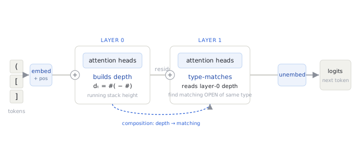
Five per-head diagnostics are computed on held-out data. Let $A^{(\ell,h)}_{t,s}$ denote the attention weight from query position $t$ to key position $s$ for head $h$ in layer $\ell$, and write $\mathcal{C}$ for the set of CLOSE positions in a sequence. Three of the diagnostics probe the QK circuit (where a head attends), one probes the OV circuit (what it writes toward the unembedding), and one probes the residual representation between layers. These are defined as follows:
Bracket-match score. For each CLOSE at position $t$, let $\mu(t)$ be the position of its unique matching OPEN (the most recent unmatched OPEN, recovered by a stack scan). The score is the mean attention a head places on the matched OPEN,
\[\mathrm{bm}(\ell,h) = \big\langle\, A^{(\ell,h)}_{t,\,\mu(t)} \,\big\rangle_{t \in \mathcal{C}}.\]Type-match score. For $k \geq 2$, a head can attend to a same-type OPEN without attending to the correct one. Writing $\tau(t)$ for the bracket type of the token at $t$, the type-match score sums attention onto all prior OPENs of the matching type,
\[\mathrm{tm}(\ell,h) = \Big\langle \textstyle\sum_{s < t}\, A^{(\ell,h)}_{t,s}\, \mathbf{1}\!\left[\,s \in \mathrm{OPEN},\ \tau(s) = \tau(t)\,\right] \Big\rangle_{t \in \mathcal{C}}.\]A head that does true matching scores high on both $\mathrm{bm}$ and $\mathrm{tm}$; a head that merely routes by type but not position scores high on $\mathrm{tm}$ alone.
Previous-token score. The mean attention from each position to the one immediately before it,
\[\mathrm{pt}(\ell,h) = \big\langle\, A^{(\ell,h)}_{t,\,t-1} \,\big\rangle_{t}.\]Copying score (OV circuit). Independently of where a head attends, does its OV circuit map a bracket token to itself or to the opposite bracket in logit space? Form the OV-to-logit map $M^{(\ell,h)} = W_E\, W_V^{(\ell,h)}\, W_O^{(\ell,h)}\, W_U$, and for each bracket type $i \in {1,\dots,k}$ take a diagonal-minus-off-diagonal contrast on that type’s $(\mathrm{O}_i, \mathrm{C}_i)$ pair, then average over types,
\[\mathrm{cp}(\ell,h) = \frac{1}{k}\sum_{i=1}^{k} \Big[\tfrac12\big(M_{\mathrm{O}_i,\mathrm{O}_i} + M_{\mathrm{C}_i,\mathrm{C}_i}\big) - \tfrac12\big(M_{\mathrm{O}_i,\mathrm{C}_i} + M_{\mathrm{C}_i,\mathrm{O}_i}\big)\Big].\]A positive value is an identity-copying OV circuit (the induction signature: promote the attended token); a negative value is a flip circuit (promote the opposite bracket), which is the task-correct readout for bracket prediction — a CLOSE should be predicted after attending to the matching OPEN. Because the readout’s job is the flip, the diagnostic readout heads in the results below carry strongly negative copying scores.
Depth correlation (residual representation). Let $z^{(\ell)}_t$ be the residual stream after layer $\ell$ at position $t$, and $\mathrm{PC}_1$ its leading principal component over all positions. The score is the absolute Pearson correlation between the projection and the ground-truth stack depth $d_t$,
\[\rho(\ell) = \big|\,\mathrm{corr}\big(\langle z^{(\ell)}_t, \mathrm{PC}_1\rangle,\ d_t\big)\,\big|.\]The first four are correlational — they say where a head looks and what its OV writes, not whether that computation is used. The patching analysis below supplies the interventional complement.
Results
Dyck-1: a bracket-flipping shortcut
For the Dyck-1 task, the two-head model reaches loss $0.5941$ against a floor of $0.5948$, with a gap of $-0.0007$ within finite-batch noise. It exhibits no induction-shaped circuitry at all. Every bracket_match score is below $0.05$ (the uniform-attention background), every prev_token score below $0.04$, and the depth correlation is $0.029$ (layer 0) and $0.044$ (layer 1) — essentially zero. Layer 1 is inert on every measure. The telling signature is the layer-0 copying scores, which are strongly negative ($-1.06$ and $-0.74$): the OV circuits project attended-OPEN representations onto -CLOSE directions. This means that the model has learned a bracket-flipping shortcut — attend diffusely to recent tokens and emit the opposite bracket type — rather than anything resembling matching. A three-head variant shows the same qualitative pattern but had not fully converged at 5000 steps, gap $+0.033$; overparameterization appears to slow optimization here, not change the solution.
Why does this suffice? Although the generating distribution depends on depth at the boundaries, only 14.4% of positions are forced; the rest are coin flips. A model can sit on the entropy floor by getting the boundary positions right, and a position-conditioned heuristic — long runs of recent OPENs imply proximity to the depth ceiling, and conversely — achieves this without tracking depth. The conclusion is not that the conjecture fails but that Dyck-1 next-token prediction is not a structural-complexity test: it is a depth-bounded random walk, and the model exploits the randomness. The refined requirement on a test language is that it demand information flow that cannot be implemented within a single layer. Dyck-1’s depth bound does not meet this bar; type matching at $k \geq 2$ does.
Dyck-2 and Dyck-3: a factored two-stage circuit
The three-head model solves Dyck-2 to gap $+0.0003$ and shows a qualitatively different circuit:
| measure | L0.H0 | L0.H1 | L0.H2 | L1.H0 | L1.H1 | L1.H2 |
|---|---|---|---|---|---|---|
| bracket_match | 0.016 | 0.079 | 0.045 | 0.070 | 0.055 | 0.001 |
| type_match | 0.27 | 0.31 | 0.28 | 0.49 | 0.49 | 0.37 |
| prev_token | 0.017 | 0.085 | 0.051 | 0.045 | 0.033 | 0.009 |
| copying | −0.09 | −0.10 | −0.07 | 0.02 | 0.07 | −0.91 |
The depth correlation is $0.747$ after layer 0 and $0.060$ after layer 1. This implies that layer 0 builds the depth representation — the leading residual-stream PC tracks running depth — while its heads attend to same-type OPENs only diffusely (type_match $\approx 0.28$). Layer 1 performs type-aware matching: two heads place nearly half their CLOSE-position attention on prior same-type OPENs, and the third (L1.H2) carries a strongly negative copying score, marking it as the candidate “predict the CLOSE of the matched type” readout.
Dyck-3 confirms the pattern at gap $+0.0034$ against the floor of $1.176$ nats. It has depth correlation $0.656$ in layer 0 and $0.060$ in layer 1, layer-1 type_match scores of $0.28$, $0.23$, $0.20$, and the negative-copying readout signature distributed across the layer-1 heads (copying scores $-0.42$, $-0.15$, $-0.35$), with the flip concentrated on L1.H0. The per-head type_match decline from Dyck-2’s $0.49$ to Dyck-3’s $0.28$ is consistent with a fixed attention budget spread over more bracket types; a model with $n_{\mathrm{heads}} \approx k$ in layer 1, allowing one head per type, is a natural follow-up I have not run.
While the canonical Olsson induction circuit copies the attended token, predicting a positive copying score; my layer-1 readouts are strongly negative. This is the correct OV for the task: at a position whose next token is $\mathrm{CLOSE}_i$, the head attends to the matching $\mathrm{OPEN}_i$ and must emit $\mathrm{CLOSE}_i$ — lookup-then-flip rather than lookup-then-copy. The circuit is structurally analogous to induction (look back, route forward) with a task-appropriate OV transformation.
Causal validation by activation patching
To obtain the causal picture beyond correlational diagnostics, I use activation patching. This involves running the model on a clean prompt and a
corrupted twin that demands a different answer, patching clean activations
into the corrupted run one location at a time, and measuring how much of
the clean prediction is recovered. I created clean and corrupted prompts of
length 10 that differ in exactly one OPEN type at position 1, with
intervening matched filler pairs leaving that OPEN unmatched at the
prediction position: ^[()()()() requires ] next, while
^(()()()() requires ). Reference logit differences are
$\pm 7.32$, averaged over 32 paired examples on the three-head Dyck-2
model.
The table below demonstrates that residual-stream patching localizes the computation sharply:
| pos 1 (swap) | pos 9 (pred) | other positions | |
|---|---|---|---|
| L0 patch | 100% | 0% | 0% |
| L1 patch | 20% | 85% | 0% |
Recovery is essentially binary: type information enters the residual stream at (layer 0, swap position), arrives at (layer 1, prediction position), and is invisible everywhere else — precisely the build-state-then-route pattern the per-head measures suggested.
I did per-head patching at the prediction position to determine which layer-1 head carries the effect; results are in the table below:
| Head | recovery | type_match | copying |
|---|---|---|---|
| L0.H0 | +79% | 0.27 | −0.09 |
| L0.H1 | −2% | 0.31 | −0.10 |
| L0.H2 | +3% | 0.28 | −0.07 |
| L1.H0 | −1% | 0.49 | +0.02 |
| L1.H1 | −2% | 0.49 | +0.07 |
| L1.H2 | +102% | 0.37 | −0.91 |
This data shows that L1.H2 alone fully recovers the clean prediction — and it is the head with the lowest type_match in its layer ($0.37$ against $0.49$) and the most negative copying score. The reconciliation is that attention statistics measure where a head looks, while the copying score measures what its OV circuit writes toward the unembedding. The functioning readout needs both adequate attention to the matched OPEN and the flip-implementing OV, and either alone is insufficient. L1.H0 and L1.H1 attend to the matched OPEN strongly but their OV does not convert that attention into the correct CLOSE logit so they are redundant pathways, auxiliary signals, or computations the model does not ultimately use. Pure attention-pattern analysis would have nominated exactly the wrong heads, patching is what surfaces the discrepancy, consistent with Wen et al. (2023) warnings about myopic interpretation of attention on Dyck. Patching at the swap position completes the picture: L0.H0 and L0.H1 recover 28% and 43% respectively there, L0.H2 only 2%, and all layer-1 heads recover exactly 0%. Layer 1 attends only backward, so its output at position 1 cannot influence position 9. L0.H0’s 79% recovery at the prediction position indicates a parallel layer-0 pathway carrying type information directly via its head output rather than through the residual PC.
Width controls factorization, not capability
Earlier I asked whether the clean one-role-per-head factorization is forced by the task or a luxury of having a spare head. The answer — it is a luxury; width controls how cleanly the circuit factorizes, not whether the task is solved — is one of the findings below. Two heads in one layer are not a substitute for two layers: they add parallel capacity at a single routing step, not a second, dependent step.
Trained on Dyck-2 for the standard 5,000 steps, the two-head model reaches a gap of only $+0.0047$ — it has not converged to the floor. Trained 4× longer (20,000 steps) it does converge, to a gap of $+0.0010$, but to a qualitatively different circuit:
| 2-head, 5k | 2-head, 20k | 3-head, 5k | |
|---|---|---|---|
| gap | +0.0047 | +0.0010 | +0.0003 |
| L0 depth correlation | 0.611 | 0.385 | 0.747 |
| L1.H0 copying | −0.67 | −0.26 | +0.02 |
| L1.H1 copying | −0.20 | −1.32 | +0.07 |
| max L1 type_match | 0.35 | 0.34 | 0.49 |
The table above shows that the converged two-head model concentrates the flip readout on a single head (L1.H1 copying $-1.32$, against $-0.26$ for its partner), much as the three-head model does, but it pays for having one fewer layer-0 head by having a markedly weaker depth representation ($0.385$ versus $0.747$), with depth tracking entangled into the same heads that do type work rather than occupying a separable principal component. The cleanly factored two-stage circuit — a clean depth PC in layer 0, a clean single flip readout in layer 1 — is therefore a property of sufficient width, not an inevitability of the task. This echoes the broader observation that larger models often exhibit cleaner, more localized and interpretable circuits because they can afford specialized heads independent of whether these additional heads are required to solve the task.
Discussion
The table below assembles the experiments, which share an architecture and differ only in data structure:
| experiment | gap | L0 depth corr. | max L1 type_match | layer 1 |
|---|---|---|---|---|
| synthetic induction¹ | +0 | n/a | n/a | dead |
| Dyck-1 | −0.0007 | 0.029 | n/a | dead |
| Dyck-2 | +0.0003 | 0.747 | 0.49 | active |
| Dyck-3 | +0.0034 | 0.656 | 0.28 | active |
¹ Deterministic given its first half, hence no entropy floor.
The data supports the conclusion that tasks solvable by single-layer shortcuts are solved by single-layer shortcuts (with layer 1 left dead), and the two-stage circuit appears exactly when the language demands it. Layer separation occurs when the language requires information flow that cannot be implemented in a single layer. Type matching at $k \geq 2$ is that minimal requirement in the Dyck-$(k, m)$ family.
The methodological lesson generalizes beyond bracket languages. Correlational head diagnostics — attention patterns, OV statistics — are necessary but not sufficient: they enumerate the circuits that might be present, but in the patching analysis of my models they nominated the wrong readout heads while assigning an unremarkable profile to the causally dominant one. Interventional methods (patching, ablation) are what distinguished the candidate circuitry from functioning circuitry.
Closing the causal chain: four follow-up experiments
The core results above leave four specific questions open, each of which can be settled with a targeted experiment on the converged models. Below I describe each question and the corresponding experiment I ran. The results of these experiments confirm the factored-circuit picture while sharpening it in two places.
1. Does layer 1 actually consume layer 0’s depth representation? The patching results show type information flowing layer-0 → layer-1, but not that layer-1’s matching specifically reads the depth PC. To test this directly, I ablated a single direction of layer-0’s output — the depth-PC1 direction — and measured the effect on layer-1 bracket-match attention, against a control that ablates a random orthogonal direction of equal norm. The depth ablation degrades layer-1 matching ($\mathrm{bm}$ on the two matching heads falls $0.068 \to 0.064$ and $0.055 \to 0.042$), while the random-direction control leaves it essentially untouched ($0.068 \to 0.068$, $0.055 \to 0.055$). The effect is modest but specific to the depth direction: layer 1’s matching heads do read layer 0’s depth representation, not merely some generic feature of its output.
2. At what width does the clean factorization set in? The two-versus three-head comparison suggested width controls factorization; sweeping $n_{\mathrm{heads}} \in {2,3,4,5,6}$ on Dyck-2 (three seeds each, $d_{\mathrm{head}}$ fixed at $32$, all trained to $8{,}000$ steps so the slower-converging widths are compared at a matched budget) shows the relationship is not monotone. Measuring how concentrated the flip readout is on a single head — the ratio of the largest $|\mathrm{cp}|$ to the sum across layer-1 heads — gives:
| $n_{\mathrm{heads}}$ | 2 | 3 | 4 | 5 | 6 |
|---|---|---|---|---|---|
| readout concentration | 0.66 | 0.80 | 0.56 | 0.58 | 0.55 |
| L0 depth correlation | 0.70 | 0.65 | 0.54 | 0.40 | 0.43 |
| seeds grokked | 3/3 | 3/3 | 3/3 | 2/3 | 3/3 |
The cleanest single-head readout occurs at three heads, and degrades on both sides — adding heads beyond three spreads the flip across the layer rather than concentrating it, and also dilutes the layer-0 depth signal across more heads (the correlation with a single PC falls from $0.70$ to $0.43$). So the clean factorization is a sweet spot matched to the task’s natural number of roles, not the top of a monotone trend; “more width gives cleaner circuits” holds only up to the point where width starts hosting redundant copies. The five-head models converged less reliably — one seed of three failed to reach the floor — but with only three seeds I draw no strong conclusion about why.
3. Does the linear depth code survive deeper nesting? At $m = 8$ the depth PC tracks ground-truth depth at $\rho = 0.74$. Retraining at $m = 16$ and $m = 32$ (with context lengths scaled to $6m$) shows the linear representation degrading as nesting deepens:
| $m$ | 8 | 16 | 32 |
|---|---|---|---|
| L0 depth correlation $\rho$ | 0.74 | 0.57 | 0.56 |
| gap | $-0.001$ | $+0.001$ | $+0.005$ |
The model keeps solving the task (the gap stays near zero), but it does so with a steadily less linear depth representation — consistent with a drift toward a compressed, logarithmic, or counter-style code once a single linear coordinate can no longer cover the dynamic range, as one would expect on information-packing grounds.
4. Do the matching heads locate their target by position or by content? Zeroing the positional embeddings at inference does not collapse layer-1 matching: bracket-match attention actually rises ($0.068 \to 0.102$, $0.055 \to 0.113$) and type-match falls only modestly (e.g. $0.50 \to 0.36$ on one head). A purely positional matcher would break when positions are removed; instead matching largely survives, so the matching is substantially content-based — driven by the type and depth content routed through the residual stream rather than by absolute position. The signal is mixed rather than clean (the modest type-match drop indicates position carries some of the matching), and the increase in raw bracket-match attention under position ablation is itself a caution against over-reading attention magnitude, but the dominant story is content-driven matching.
Limitations
Two caveats survive these follow-ups. The depth-saturation and factorization sweeps are small (three seeds, a single $k$), enough to show the qualitative trends above but not to pin the exponents or thresholds precisely; the five-head reliability dip in particular wants more seeds before it means anything. The related work in §1 implies that several of these observations plausibly reproduce known results, and a systematic comparison against the constructions of Yao et al. (2021) and the multiplicity results of Wen et al. (2023) is owed before any novelty claim. The results in this post are presented as a self-contained empirical study, not a claim of priority.
Reproducibility
All experiments run on a single Apple M3 Pro chip — an Arm system-on-chip with a 12-core CPU (6 performance + 6 efficiency cores) and an 18-core integrated GPU sharing 18 GB of unified memory, with PyTorch on the Metal Performance Shaders (MPS) backend rather than CUDA. Training scripts,
per-head diagnostic implementations, and patching utilities are in
interp-repo; the executed analysis notebooks
are notebooks/dyck/explore.ipynb (Dyck-1),
notebooks/kdyck/explore.ipynb (Dyck-2/3).
Prose edited with the assistance of Claude (Anthropic), which also checked the numbers against the analysis artifacts and ran supplementary experiments. I ran the main experiments and vouch for every claim here.