Introduction

Grokking is a well known phenomenon in neural networks where models exhibit an abrupt transition to a generalizing solution despite initially overfitting. This occurs long after the training loss has flatlined and is one of the cleanest examples of a phase transition occurring during training. Grokking was first reported by Power et al. (2022) when training a decoder only transformer on modular arithmetic. Subsequently, Nanda et al. (2023) reverse-engineered the Fourier-multiplication circuit behind the generalizable solution. Since then, many additional studies have attempted to explore the conditions in which grokking occurs and uncover mechanisms to explain why it happens.

A great deal of grokking work fixes the architecture and the train/test split at a single fixed fraction and studies the learning dynamics there. However, the learning dynamics depend strongly on whether the train/test split sits relative to the capacity of the network. The canonical “memorize-first, generalize-late” phenomenon is only one of several regimes. The simplest way to see this is to train with different train test fractions set by scaling the size of the network, and the value of the modulus $p$.

In prior work, Liu et al. (2022) mapped a four-phase diagram (comprehension, grokking, memorization, confusion) on modular arithmetic and noted the existence of a small-decoder regime that does not grok. Varma et al. (2023) explained the late switch through circuit efficiency — weight decay favoring a norm-efficient generalizing circuit over a memorizing lookup. Huang et al. (2024) drew the 2D phase diagram over model size and dataset size, and found a small-model regime of immediate generalization.

In this post I reproduce grokking in the task of modular addition from scratch across a grid of model widths and training fractions. I recover the phase structure that has appeared in several parts of the literature and analyze it through the same finite-size-scaling lens I have been applying to circuit formation and to emergence elsewhere on this blog. I treat the critical training requirement as a finite-size-scaling problem in the modulus $p$ and ask which rescaling of the data axis — fraction, absolute count, or coverage — collapses the onset across moduli, attempting to isolate a single critical fraction.

Code and executed notebooks: interp-repo.

Setup

The task I study is modular addition $a + b \bmod p$ in a one-layer transformer with 4 heads, ReLU MLP trained with full-batch AdamW, and weight decay $1.0$. This is the same setup used by Nanda et al. (2023) except that I train for up to $40{,}000$ epochs. I chose this number by previously observing the timing of the grokking transition for 10 seeds. During training, the model sees a fixed fraction of the $p^2 = 12{,}769$ possible pairs as its training set and is evaluated on the held-out remainder. In the initial experiments, I varied the width and train fraction, keeping other parameters fixed. I defined the width of the network to be the embedding/residual dimension and the train fraction as the share of pairs in the training set. In this setup the width is a proxy for model capacity: networks with larger $d$ can memorize more pairs as a lookup table. Likewise, the size of the training set determines the amount of data the model has to memorize to fit the training set. I chose $d \in {16, 32, 64, 128, 256}$ and $f \in {0.2, 0.3, 0.4, 0.5, 0.6}$.

I run three seeds for each pair of values of $d$ and $f$ for a total of $5 \times 5 \times 3 = 75$ runs. For each run I log the full train/test accuracy trajectories and read off three quantities: the presence of a grokking transition (using the working definition of the test accuracy crossing $0.95$ within the budget), the epoch at which grokking occurs (if it does), and the memorization delay defined as the gap in epochs between the train accuracy crossing $0.95$ and the test accuracy reaching that value. The delay is the quantity that distinguishes the regimes: a large delay is the classic memorize-then-generalize picture; a near-zero delay means train and test rose together, with no separate memorization phase to grok out of.

Everything below regenerates from the training script (scripts/train_grokking.py) and the committed per-run statistics; no GPU is needed to reproduce the analysis.

The phase diagram

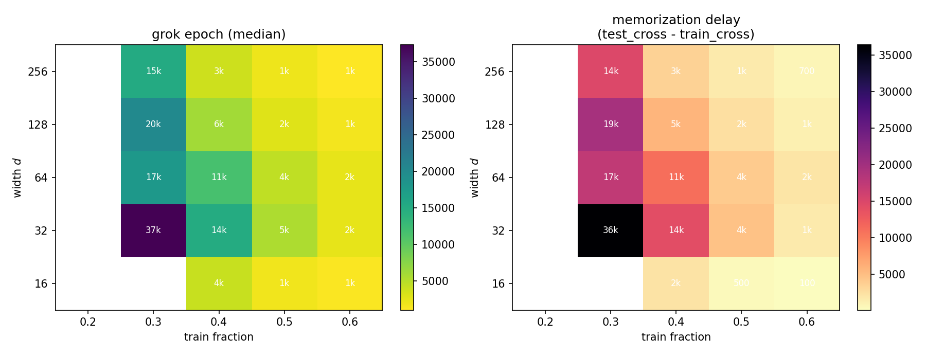
In the heat maps above, the right panel shows the memorization delay.

The data-fraction axis dominates, and there is a sharp lower edge At $f = 0.2$ nothing groks, at any width: the model memorizes the training set (train accuracy reaches $1$) but test accuracy never follows within the budget. This is the data-poor regime — below a task-and-model-dependent critical fraction, delayed generalization simply does not occur, consistent with the critical-data-size picture of Zhu et al. (2024). As $f$ increases the delay collapses by more than two orders of magnitude, from tens of thousands of epochs down to a few hundred.

The capacity axis sets the boundary at the critical fraction The $f = 0.3$ column is the transition zone, and it is where width matters most. At small width ($d = 16, 32, 64$) only a minority of seeds grok; at large width ($d = 128, 256$) all of them do. Capacity controls whether grokking occurs at the critical data fraction and how long it takes to happen.

Small capacity compresses the delay For $d = 16, f = 0.3$: train accuracy there does not cross $0.95$ until $\sim 11{,}000$ epochs, against $100$–$700$ for every larger model. The smallest network at the critical fraction can barely memorize the training set — it is near its capacity limit. When the smallest models do grok (e.g. $d = 16, f = 0.4$), they show the smallest delay in their column. This is because the memorization shortcut is not cheaply available. When networks are near capacity, memorization is slow and it no longer wins the race by a wide margin.

Four regimes, one trajectory each

I plot one representative seed from each corner of the plane to show the four types of trajectories.

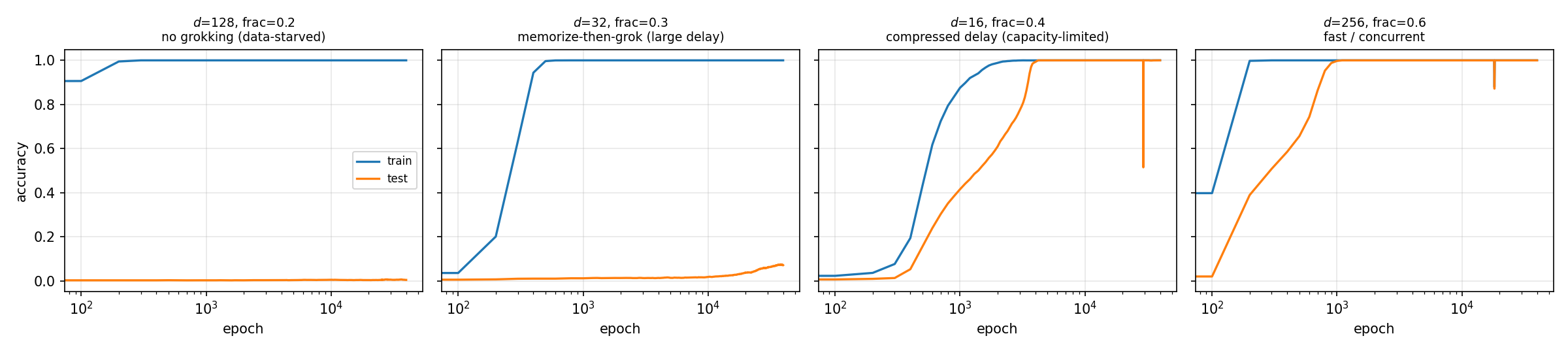
• No grokking ($d = 128, f = 0.2$): train accuracy saturates and test accuracy sits at chance. There is capacity but too little data — the model memorizes and stops.
• Memorize-then-grok ($d = 32, f = 0.3$): Train accuracy hits $1$ early, but test accuracy languishes for tens of thousands of epochs, then jumps with a long flat gap between the two curves.
• Compressed delay ($d = 16, f = 0.4$): train and test rise almost together. There is still a gap, but a small one — a capacity-limited model cannot race ahead on memorization, so the two phases nearly merge.
• Fast / concurrent ($d = 256, f = 0.6$): ample capacity, ample data; the model generalizes about as soon as it fits, with only a short delay.

The canonical grokking examples in the literature are usually located in the memorize-then-grok regime. The width of the valley between memorization and the onset of grokking is widest in a narrow band of the (capacity, data) plane and shrinks to nothing on either side.

Grokking as a finite-size transition

I now study the memorization delay as a function of width and data fraction, and show that the emergent jump in test accuracy is not an intrinsic constant but depends strongly on both — and, as the next section shows, on the modulus $p$.

Under this lens the competing explanations stop reading as rivals. Circuit efficiency (Varma et al.) explains why the generalizing solution eventually wins; the critical-data-size picture (Zhu et al.) explains the lower edge in $f$; the speed-competition account (Song & Ye) explains why the boundary bends with capacity and why small models compress the delay. Each describes a different feature of the same surface. Drawing the surface shows they are local descriptions of one global phase structure.

How to scale the training set

Power et al. (2022) and Nanda et al. (2023) set the absolute size of the training set as a fraction $f$ of the $p^2$ possible pairs, which I followed for my initial runs. They quote a critical fraction (for modular addition, $f_c \approx 0.25$–$0.3$) as if it were a property of the task. However, as $p$ changes, the same fraction $f$ corresponds to a different amount of data relative to the size of the model.

Nanda et al. (2023) showed that the generalizing solution is a Fourier-multiplication algorithm built on a handful of key frequencies; Liu et al. (2022) characterized the critical training set as the least data that pins down that representation. However, that is a statement about a count of constraints, not a fraction. How the required amount of training scales with $p$ is an empirical question. Fixing $f$ assumes that it should be $p^2$. However, if the structure is fixed by $O(p)$ or $O(p\log p)$ relations, then holding $f$ constant across $p$ does not define the phase boundary.

Which rescaling of the data axis makes the threshold $p$-independent? The most obvious candidates are

• fraction $f$ — implying the requirement scales as $p^2$.
• Absolute pairs $N = f\,p^2$ — implying a fixed number of examples suffices regardless of $p$.
• Coverage $N/p = f\,p$ — how many times each residue appears in the training set; a fixed coverage means each symbol is seen a constant number of times, so the requirement scales as $p$.

These predict different motions for $f_c(p)$. A fixed $N$ would need $f_c > 1$ at $p = 31$, which is impossible, so a fixed count is too strong and the requirement grows sub-quadratically. If coverage is invariant, $f_c$ should scale as $1/p$; if the fraction is invariant, $f_c$ should be flat.

I rerun the onset measurement at seven moduli, $p \in {31, 41, 47, 53, 59, 79, 113}$, sweeping the train fraction at each to locate $f_c(p)$ — the fraction at which the median seed first groks within budget — and ask which axis, $f$, $N$, or $N/p$, collapses the seven onset curves onto one.

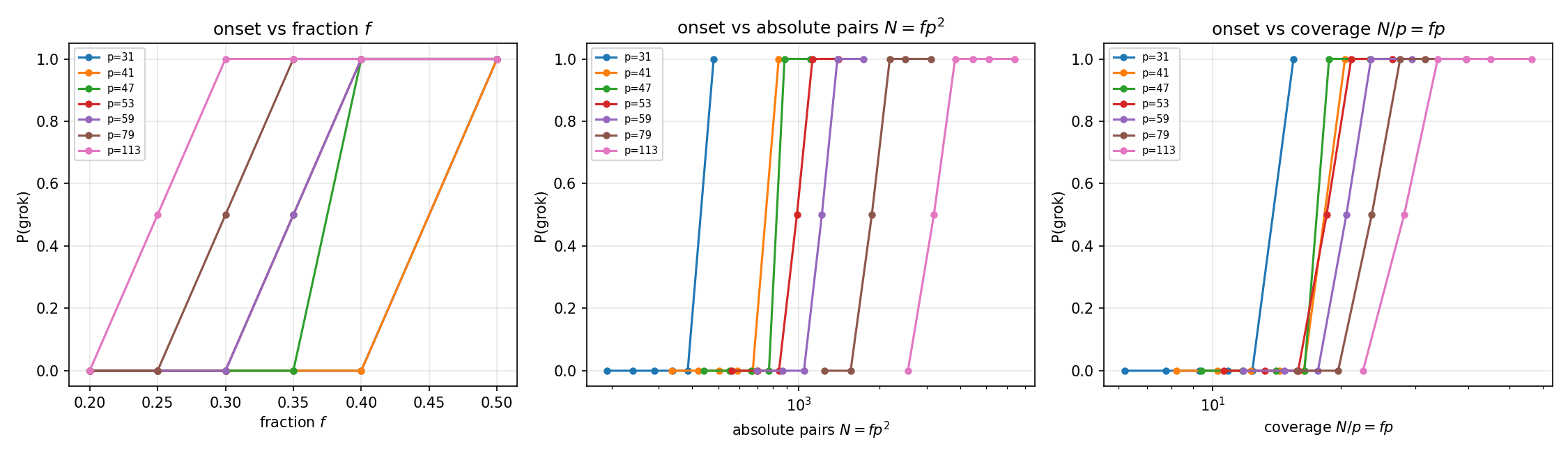
The collapse rules out both a fixed fraction and absolute pairs. The critical fraction is not constant: it runs from $f_c = 0.5$ at $p = 31$ down to $f_c = 0.25$ at $p = 113$, halving across the range (left panel — the onset curves fan out, ordered by $p$). So a single quoted critical fraction is genuinely $p$-dependent. Absolute pairs $N$ is too demanding: the middle panel spreads the curves wider still, and a fixed $N$ would require $f_c > 1$ at the smallest prime. Coverage $N/p$ (right panel) brings the curves closest together of the three — the best simple variable — but it slightly over-corrects, and the onsets do not perfectly stack.

Fitting the exponent gives the scaling:

\[f_c(p) \sim p^{-0.58},\]

which is close to $p^{-1/2}$, between a $p$-independent fraction-invariance ($p^{0}$) and coverage ($p^{-1}$). In terms of a constraint count, the critical number of pairs is

\[N_c = f_c\,p^2 \sim p^{2 - 0.58} \approx p^{3/2},\]

$N_c$ runs $480, 840, 884, 983, 1218, 1872, 3192$ across the seven primes — faster than coverage ($\sim p$), slower than a fixed fraction ($\sim p^2$). The data requirement for grokking modular addition grows like $p^{3/2}$: neither “a constant fraction of all pairs” nor “each symbol a constant number of times,” but between them.

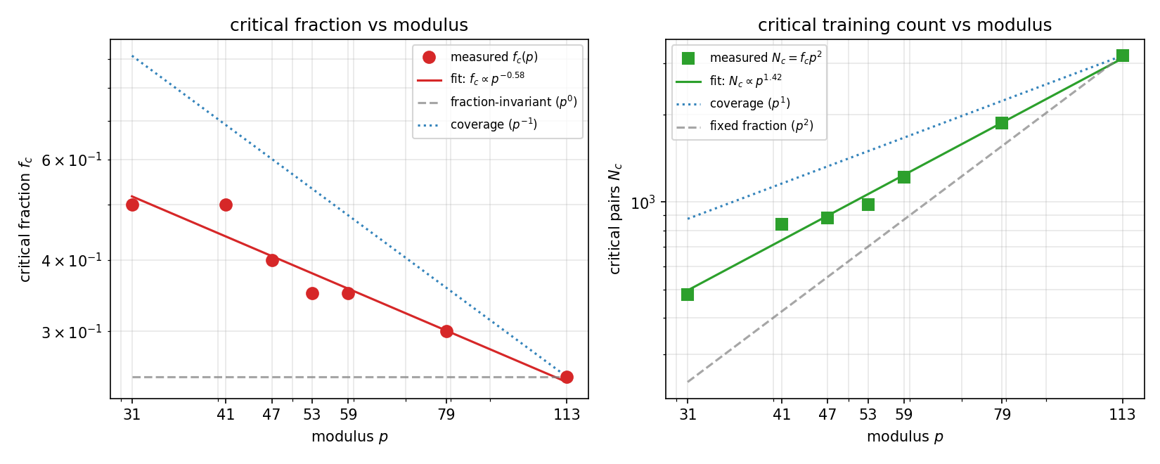
I plot $f_c(p)$ on log–log axes and fit the points to a line to obtain an approximate value for the scaling exponent. The left panel places $f_c(p)$ between the flat fraction-invariant slope and the steeper $p^{-1}$ coverage slope; the right panel puts the critical count $N_c$ on $p^{1.42}$, bracketed by coverage ($p^{1}$) and fixed fraction ($p^{2}$).

I test the $p^{3/2}$ scaling by plotting the onset against the rescaled axis $N/p^{3/2}$ and see that the seven per-prime curves collapse onto one.

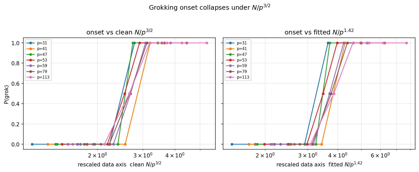
The left panel uses the clean $3/2$, the right the fitted $1.42$. Both stack the seven onset curves into a single step crossing $P(\mathrm{grok}) = \tfrac12$ in a narrow band near $N/p^{3/2} \approx 2.7$. The $p^{3/2}$ count is about what one expects if the Fourier solution needs of order $p$ constraints to fix its key frequencies and a further $\sqrt{p}$-like redundancy to win the optimization race against memorization, but that requires further study to confirm.

Overall this shows that the train fraction is the wrong control variable for the phase diagram and that reporting grokking thresholds as fractions — without saying at which $p$ and which capacity — bakes in a $p^2$ scaling the data do not obviously support. It is the same move as the finite-size-scaling collapses that fold a family of rounded transitions onto one universal curve; here the “size” is the modulus and the control variable is how much of the group table the model has seen.

Discussion

I mapped grokking on modular addition across the (capacity, data-fraction) plane and recovered the phase structure that has appeared piecemeal across the literature. The data-fraction axis dominates: below a critical fraction nothing groks at any width, and above it the memorization delay collapses by more than two orders of magnitude. Capacity sets the boundary at that critical fraction and controls how the delay behaves — models with ample capacity race ahead on memorization and grok late, while models near their capacity limit cannot take the memorization shortcut cheaply and so generalize almost as soon as they fit. The four canonical regimes (no grokking, memorize-then-grok, compressed delay, fast/concurrent) are corners of this single surface, and the competing explanations — circuit efficiency, critical data size, and the speed-competition account — each describe a different feature of it rather than standing as rival mechanisms.

The central result is that the train fraction is the wrong control variable for the phase boundary. The critical fraction is not a property of the task: it runs from $f_c = 0.5$ at $p = 31$ down to $f_c = 0.25$ at $p = 113$, scaling as $f_c(p) \sim p^{-0.58} \approx p^{-1/2}$. Read as a constraint count this is $N_c \sim p^{3/2}$ — faster than coverage ($\sim p$), slower than a fixed fraction ($\sim p^2$) — and rescaling the data axis by $N/p^{3/2}$ collapses the seven per-prime onset curves onto a single step. Reporting a grokking threshold as a fraction without naming $p$ and the capacity therefore bakes in a $p^2$ scaling the data do not support; the natural “size” for a finite-size-scaling treatment is the modulus, and the right control variable is how much of the group table the model has seen.

I read these results as suggestive rather than settled — the grid is coarse and the $p$-collapse spans less than a decade in $p$ — but the direction is consistent across all seven moduli.

A recent information-theoretic account (Song & Ye, 2026) argues that grokking onset is not a static capacity threshold at all but a race between a memorization timescale and a generalization timescale, both functions of model size — a refinement that complicates the simple threshold reading. That race unfolds along the optimization-time axis, complementary to the data-axis rescaling I study here. The critical data requirement governs whether the generalizing circuit is reachable at all, while the competing timescales govern how quickly it is reached. Reading the onset from late-time accuracy, as I do, folds the two effects together.

Reproducibility

All experiments run on a single Apple M3 Pro chip — an Arm system-on-chip with a 12-core CPU (6 performance + 6 efficiency cores) and an 18-core integrated GPU sharing 18 GB of unified memory, with PyTorch on the Metal Performance Shaders (MPS) backend rather than CUDA. The training script, the $75$-run sweep, the committed per-run statistics, and the analysis that produces every figure are in interp-repo, with the executed notebook alongside.

---

Prose edited with the assistance of Claude (Anthropic), which also checked the numbers against the analysis artifacts and ran supplementary experiments. I ran the main experiments and vouch for every claim here.