Introduction

Comparing the SARSA and Q-learning algorithms used to train an agent to walk on a cliff environment is a rite of passage when learning RL. The textbook result shows that the learned SARSA policy results in the agent taking the safe path far from the edge and the Q-learning policy results in the agent taking the optimal-but-risky path on the edge of the cliff. These algorithms differ only in which next-state action-value enters the bootstrap target — both still behave the same $\varepsilon$-greedy way. The usual demonstration runs SARSA and Q-learning on separate sets of trajectories, which mixes algorithmic and initialization effects together. To isolate them, the experiment has to control for initialization and exploration at once.

In this post I compare the SARSA and Q-learning algorithms by properly controlling for initialization and exploration. I find the difference resolves into two numbers that should be considered separately: SARSA earns the higher behavior return by exploring at a safe distance from the cliff, while Q-learning reaches the better greedy policy ($-12$ vs $-16$) because its target ignores the cost of exploration. The real payoff is a confound-free comparison of the two update rules — not variance reduction, which washes out of the run total here.

Code and executed notebooks: rl-alignment-repo.

Related work. The cliff-walking task is Example 6.6 of Sutton & Barto; what follows is a methodological re-examination of a standard example. Pairing runs with common random numbers is a classical variance-reduction technique from simulation; in reinforcement learning it appears as the fixed-seed value estimate of PEGASUS (Ng & Jordan, 2000) and is used explicitly for variance reduction in TRPO (Schulman et al., 2015). That RL comparisons are highly sensitive to the choice of seed, and that reporting interval estimates over many runs rather than single trajectories is the honest alternative, is argued forcefully by Henderson et al. (2018) and Agarwal et al. (2021).

The cliff

The cliff-walking gridworld (Sutton & Barto, Example 6.6) is a $4 \times 12$ grid, where the agent starts at a state $S$ at the bottom-left and attempts to reach a goal state $G$ at the bottom-right. The entire bottom row between $S$ and $G$ is a cliff, which the agent must learn to avoid. The agent can take four deterministic actions (up/down/left/right) where every step that does not go over the cliff costs $-1$. Stepping into the cliff costs $-100$ and teleports the agent back to $S$. Episodes are undiscounted ($\gamma = 1$) and end when the agent reaches $G$, where the terminating transition carries reward $0$. So a path of $L$ moves returns $-(L-1)$ — one smaller in magnitude than the Sutton & Barto bookkeeping, where the final step into $G$ also costs $-1$. I use this convention throughout, so the optimal edge path scores $-12$, not the textbook $-13$.

The shortest route runs one row above the cliff — up once, right eleven times, down once — for a return of $-12$. The catch is that this optimal path hugs the cliff: one wrong step down and the agent pays $-100$. Staying safe means climbing further from the edge and paying for the extra length — the tension the SARSA and Q-learning algorithms resolve differently.

One TD error, two backups

Both Q-learning and SARSA are tabular TD(0) control algorithms. They differ only in the selection of the bootstrap target. Writing the temporal-difference error $\delta_t$ gives the following expressions for $\delta_t^{\,\mathrm{SARSA}}$ and $\delta_t^{\,\mathrm{Q}}$:

\[\delta_t^{\,\mathrm{SARSA}} = r_{t+1} + \gamma\, Q(s_{t+1}, a_{t+1}) - Q(s_t, a_t)\] \[\delta_t^{\,\mathrm{Q}} = r_{t+1} + \gamma\, \max_{a} Q(s_{t+1}, a) - Q(s_t, a_t)\]

with the common update

\[Q(s_t,a_t) \leftarrow Q(s_t,a_t) + \alpha\, \delta_t\]

While SARSA bootstraps from $a_{t+1}$, the action the behavior policy will actually take next, Q-learning bootstraps from the greedy value, pretending the agent will act greedily next regardless of what it actually does. This means that SARSA’s target carries the cost of exploration while Q-learning’s does not.

This results in SARSA evaluating and improving the policy it actually follows — the $\varepsilon$-soft policy — and reaching the optimal $\varepsilon$-soft policy as a fixed point. By contrast, Q-learning reaches a fixed point corresponding to the optimal greedy policy, independent of how it behaves. The cliff is simply a place where those two fixed points visibly disagree, because the optimal $\varepsilon$-soft policy keeps a safety margin away from the $-100$ region that the greedy optimum drops.

Asymptotic comparison

With a fixed $\varepsilon > 0$, Q-learning’s greedy policy converges to the cliff-edge optimum ($-12$), while SARSA’s settles on the maximally cautious route along the top row ($-16$): at $\varepsilon = 0.1$ the per-step cost of being cliff-adjacent, $\approx \tfrac{\varepsilon}{4}\times 100 = 2.5$, is large enough that its optimal $\varepsilon$-soft policy backs all the way off the edge. With the constant $\alpha = 0.5$ used here, neither set of $Q$-values literally converges — they reach a stationary distribution of $O(\alpha)$ width around the fixed point — but the greedy policy stabilizes well before the values stop fluctuating, which is why I read the asymptotic numbers off greedy rollouts rather than the running values. However, the quantity usually studied is the online return — the sum of rewards collected while behaving $\varepsilon$-greedily. There, SARSA wins: it rarely falls, while Q-learning walks the edge and occasionally falls off, incurring a cost of $-100$.

The subtlety is worth stating explicitly: “SARSA is safer” is a claim about learning under sustained exploration, not about the asymptotic policy. If $\varepsilon$ is annealed to $0$, both SARSA and Q-learning converge to the same greedy optimum and the gap between their expected rewards closes. But unless behavior return and greedy-evaluation return (defined below) are kept separate, the two results get conflated.

Shared seeds do not imply shared exploration

Cliff-walking has deterministic transitions, so the randomness lives entirely in three places: the $Q$-initialization, the $\varepsilon$-greedy exploration draws, and tie-breaking among equal-value actions. Two common flaws in analysis are:

Under-control. Seed one global RNG, run SARSA, then run Q-learning. They consume random numbers at different rates and in different states, so after the first step where their policies differ, their streams are effectively unrelated. So using the same seed guarantees nothing about whether the two agents faced the same exploration.

Not enough trials. A single seed is one sample, and the cliff is high-variance — a couple of unlucky falls swing the online return by tens of points. One run can make either algorithm look better by chance.

The fair experiment

Two steps reconcile these issues. First, isolate randomness into named streams so each source is reproducible and independently ablatable — one generator for initialization, one for exploration, one for tie-breaking, spawned from a single SeedSequence. Second, pair the two algorithms with common random numbers (CRN) so for each seed, SARSA and Q-learning receive the same init and exploration streams. They begin in identical states and share exploration draws up to the first policy divergence.

This is the classic variance-reduction trick. The estimand is the gap $\Delta = R_{\mathrm{S}} - R_{\mathrm{Q}}$, and

\[\mathrm{Var}(\Delta) = \mathrm{Var}(R_{\mathrm{S}}) + \mathrm{Var}(R_{\mathrm{Q}}) - 2\,\mathrm{Cov}(R_{\mathrm{S}}, R_{\mathrm{Q}}).\]

In principle, sharing randomness makes $\mathrm{Cov}(R_{\mathrm{S}}, R_{\mathrm{Q}})$ positive and shrinks the variance of the difference without biasing it — free variance reduction for the exact quantity of interest. How much you actually get depends on how long the shared randomness survives, and on the cliff that is the interesting part.

In practice the cancellation is limited. CRN synchronizes the streams only until the policies diverge, and on the cliff they diverge early and stay diverged — after that the two agents visit different states and consume the shared draws in different contexts. Measured directly, paired over master seeds, the per-episode correlation is modest ($\rho \approx 0.25$) and falls to essentially zero in the run-total online return: a run sums hundreds of episodes, the shared randomness couples the two agents only in the short pre-divergence window of each, and so each run-total averages over many near-independent trajectories. The variance reduction on the quantity I actually plot is therefore small — expected, and not the reason to pair. The reason is the part that does not depend on the cancellation surviving: pairing removes the differing-exploration confound by construction, so the gap $\Delta$ is a clean comparison of the two update rules at matched exploration rather than an artifact of one agent happening to explore into the cliff more often. With enough seeds the gap converges to the same value either way — pairing just makes each comparison honest, which is what a controlled experiment is for.

In this experiment I use the same $\alpha$, $\varepsilon$, number of episodes, same initialization of $Q$, and the same environment for both algorithms. The only difference between the Q-learning and SARSA runs comes from the greedy versus the on-policy selection of $a_{t+1}$ in the Q update. I then average over many seeds (the cliff requires $M \gtrsim 100$ for clean bands), and report a 95% confidence band rather than a single curve. Finally, I evaluate the learned greedy policies separately with greedy rollouts at $\varepsilon = 0$ so the asymptotic path is reported distinctly from the behavior return.

The core of the experiment

The whole comparison rests on one detail: at every step both algorithms draw the next action $a_{t+1}$ from the same exploration stream, so the two runs stay coupled (common random numbers) and differ only in which value enters the bootstrap target — the on-policy $a_{t+1}$ for SARSA, the greedy $\max_a$ for Q-learning.

# a2 is drawn every step in BOTH algorithms, from a shared exploration
# stream, so the paired runs stay aligned (common random numbers)
a2 = egreedy(Q, s2, eps, rng_explore, rng_tie)
if algo == "sarsa":
    target = r + gamma * Q[s2[0], s2[1], a2] * (not done)    # on-policy a_{t+1}
else:  # q-learning
    target = r + gamma * Q[s2[0], s2[1]].max() * (not done)  # greedy value
Q[s[0], s[1], a] += alpha * (target - Q[s[0], s[1], a])

The full implementation — the named RNG streams spawned from a single SeedSequence, the paired-seed loop over $M = 100$ seeds, greedy evaluation at $\varepsilon = 0$, and the figure code — is in the notebook.

Results

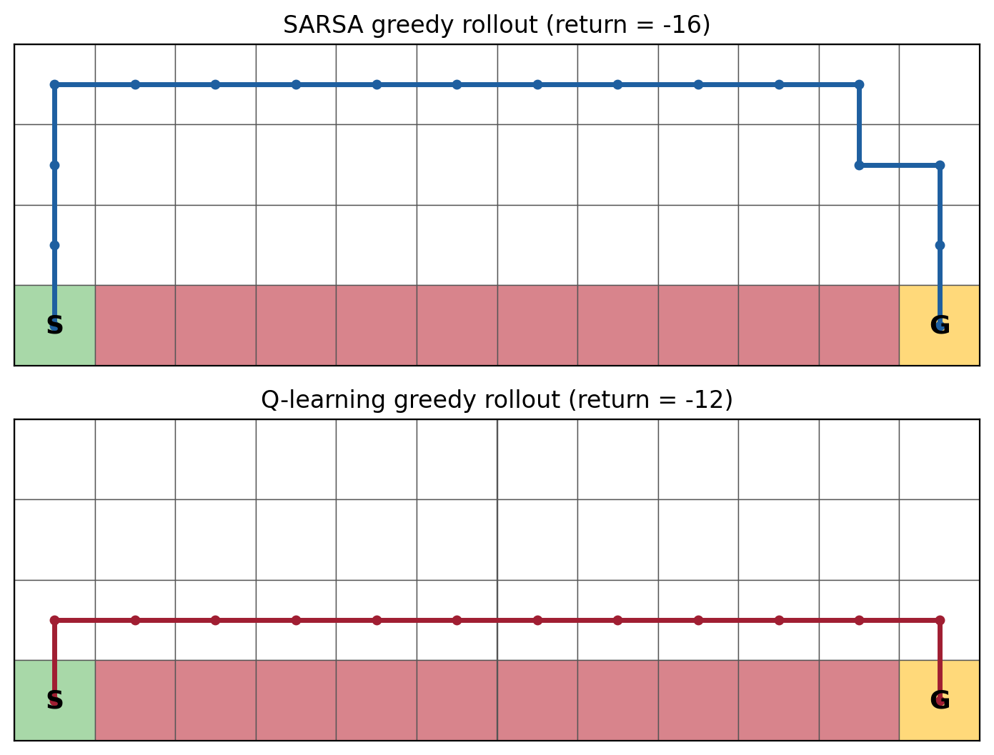
Greedy policies after 500 episodes (seed 0). Q-learning takes the cliff-edge optimum ($-12$); SARSA backs all the way to the top row and accepts the longer route ($-16$) to stay clear of the $-100$ region. The policies differ exactly where the greedy and $\varepsilon$-soft optima disagree.

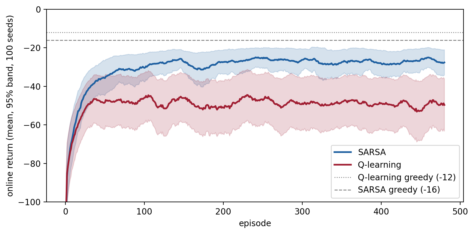
Online return during training, mean over 100 CRN-paired seeds with 95% bands. SARSA settles higher (around $-28$) because it rarely falls; Q-learning sits lower (around $-50$) as it walks the edge and occasionally steps off. The dotted and dashed lines mark the two greedy-evaluation returns ($-12$ and $-16$) — far above the behavior return, which carries the cost of exploration.

Two returns are in play and they should be compared separately. The behavior return is the reward actually collected while the agent acts $\varepsilon$-greedily during training — exploration costs and cliff-falls included; this is the online return plotted above (≈ $-28$ for SARSA, ≈ $-50$ for Q-learning). The greedy-evaluation return is the final learned policy run greedily at $\varepsilon = 0$, with no exploration ($-16$ for SARSA, $-12$ for Q-learning). SARSA earns the higher behavior return because its policy keeps a margin from the cliff: an $\varepsilon$-greedy exploratory step from a safe row is usually just a $-1$ detour, so few episodes carry a $-100$ fall. Q-learning walks the cliff edge, where a single random step often drops into the $-100$ region — so more episodes include a fall, and those penalties drag its episode-averaged return down (the $\approx \tfrac{\varepsilon}{4}\times 100 = 2.5$ per-step cliff-adjacency cost from before, now paid along the whole edge). The greedy-evaluation return flips the ranking: Q-learning wins it because its target values the greedy policy regardless of how the agent behaves. Both are correct; they answer different questions.

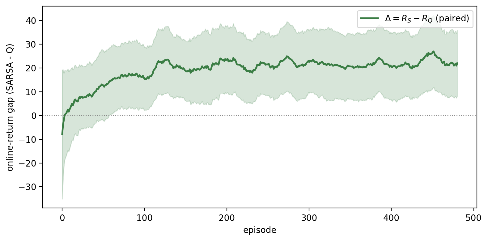
The paired gap $\Delta = R_{\mathrm{S}} - R_{\mathrm{Q}}$ in online return, mean over 100 seeds with a 95% band. It sits above zero through training — SARSA’s behavior-return advantage — but the band stays wide: pairing fixes the exploration confound without buying much variance reduction on this quantity, since the per-episode coupling washes out of the run total.

Takeaways

The algorithmic gap between SARSA and Q-learning is one symbol — max versus the on-policy $a_{t+1}$ — and it maps cleanly onto “value the greedy policy” versus “value the policy you actually run, exploration and all.” The empirical gap on the cliff is real but it is a statement about learning under sustained exploration, and it dissolves as $\varepsilon \to 0$.

In general, for a clean comparison of two RL algorithms: first isolate randomness into named streams; then pair the algorithms with common random numbers so the comparison is about the update rule and not the random number drawn; then average over many seeds and report intervals; and finally, keep behavior return and greedy-evaluation return as separate columns. “Same seed” is table stakes, not a guarantee — and pairing’s real dividend is a clean comparison at matched exploration, not the variance it happens to save.

The full analysis — the common-random-numbers coupling modes, the first-divergence diagnostic, the annealing/GLIE study of when SARSA’s greedy policy actually shortens, and the minimum-exposure solution set SARSA samples from — is in the tabular-control notebook.

Prose edited with the assistance of Claude (Anthropic), which also checked the numbers against the analysis artifacts and ran supplementary experiments. I ran the main experiments and vouch for every claim here.