Introduction

The linear representation hypothesis states that a model encodes high-level concepts as directions in activation space. This reduces reading a concept to a dot product with a single vector, and steering along it to adding a multiple of that vector to the residual stream. Marks & Tegmark (2023) showed that in sufficiently large models, a linear direction corresponding to an abstract notion of truth emerges that applies across diverse sets of inputs. They estimated this direction with a difference-in-means (“mass-mean”) direction fit on true/false statements and showed that it separates held-out statements, transfers across datasets, and is causally implicated under intervention.

Previously, Burns et al. (2022) had proposed finding a linear truth direction without labels, by demanding logical consistency, a method they call Contrast-Consistent Search (CCS). However, Roger (2023) showed empirically that the CCS estimator insufficiently constrained. Untrained, randomly initialized probes already reach about \(75\%\) accuracy on the “easy” dataset once the CCS convention of inverting the sign of a below-chance probe is applied. More than twenty mutually orthogonal “truth probes” reach accuracies similar to the one returned by the CCS estimator implying that CSS has not found the optimal linear probe. Additionally, due to the inversion convention in choosing the sign, comparing to a random baseline is misleading because the accuracy of this baseline will always be either greater than or equal to one half. Furthermore, Farquhar et al. (2023) then showed that because arbitrary binary features are optimal under that consistency loss, nothing in it selects for knowledge, and in practice unsupervised probes recover whatever feature is most prominent in the representation implying that in the unsupervised case a linear direction can appear to decode truth while actually corresponding to a salient direction that happens to correlate with the label on the particular dataset. Thus the common thread across these observations implies that the decoding of truth inherits a signal-versus-noise problem, which I will show is also relevant for the supervised case. Consequently, on a benchmark where chance-level structure is this strong, the ability of a truth probe to separate the classes is a much weaker result than it first appears.

A mass-mean “truth direction” is an estimator for the decodable truth direction which separates true and false statements. However, in the low signal-to-noise regime, it can also end up returning the most salient direction in activation sapce, i.e. the direction of largest within-class variance. On a dataset where the class gap is small relative to the within class spread along the axis connecting the centroids, the finite-sample mean difference is dominated by noise along that axis, aligning the estimator along the salient axis regardless of whether it has large overlap with the recoverable truth direction. On counterfact, the decodable truth direction does not lie along the salient axis, so the estimator returns a nuisance direction. A truth direction and a salient axis look alike on a benchmark and require a signal-to-noise reading to tell them apart. This post takes up the question of recoverability: when does a model contain a linear truth direction a probe can actually recover, which rises above a random-direction null and carries signal beyond the single most salient axis?

Systems neuroscience has spent decades asking what a downstream reader can recover from a population of noisy neural units. In that spirit I treat probing for a truth direction as a readout problem: I take the probe as a linear readout, quantify its separation with a detection-theoretic \(d'\), and benchmark that \(d'\) against an explicit random-direction null across the Pythia scale ladder. This reading yields three results:

(1) Apparent separation is trivial. Two effects inflate a probe’s score before any truth content enters. Fitting below Cover’s capacity (\(N \ll 2d\) throughout) buys separation from shuffled labels alone, and a random direction inherits a share of the real class gap, so the chance level rises with the very separation being measured. The null, not the raw score, is the bar.

(2) The estimator returns a nuisance direction when the signal is weak. It returns the dominant activation axis \(\hat v_1\) rather than a truth direction, and steering along what it returns then moves behavior with the wrong sign. Recoverability comes down to whether the class gap grows with depth until it dominates the spread along that axis. On cities it does, on counterfact it never does. That pattern, the alignment to \(\hat v_1\) and the decoding alike, replicates on OLMo-2-1B across a different architecture and corpus. The steering measurement is on Pythia alone.

(3) The failure is in the estimator, not the model: the offending direction is identified in advance from the within-class spectrum, not from the steering outcome. Removing it, without leaving the linear class, raises the held-out AUROC above the random decoding null and corrects the sign of the steering behavior, at the same layer.

Notation

I start by fixing a model and a layer \(L\). Each statement is passed through the model once and summarized by the residual-stream activation at its final token, \(x \in \mathbb{R}^{d}\), where \(d\) is the model’s hidden width. Each statement carries a truth label \(y \in \{0, 1\}\) and a dataset consists of \(N\) such pairs \((x_i, y_i)\).

Throughout, a hat marks a quantity estimated from a finite sample, and its absence marks the population quantity it estimates, with expectations taken over the data-generating distribution of activations at the probed layer. A table of every symbol used in the post is collected in the notation appendix. The distinction is crucial: almost every trap in this post is the gap between an estimate and its population target, \(\hat\theta\) and \(\theta\), or the eigenvalues of \(\hat C\) and of \(\Sigma\), which agree only in the large-sample limit. Estimates are computed on a training split of \(N_{\text{train}} = N_0 + N_1\) activations, \(N_0\) of them with \(y = 0\) and \(N_1\) with \(y = 1\). Held-out data is used only to evaluate a fitted direction, never to determine it. I define the population class means and their estimators as

\[\mu_0 = \mathbb{E}[x \mid y=0], \qquad \hat\mu_0 = \frac{1}{N_0}\sum_{i:\,y_i=0} x_i .\] \[\mu_1 = \mathbb{E}[x \mid y=1], \qquad \hat\mu_1 = \frac{1}{N_1}\sum_{i:\,y_i=1} x_i .\]

I define the class-mean gap as \(\delta = \mu_1 - \mu_0\), with \(\hat\delta = \hat\mu_1 - \hat\mu_0\), and the within-class covariance as the class-weighted average of the two class-conditional covariances,

\[\Sigma \;=\; \pi_0 \operatorname{Cov}[x \mid y=0] \;+\; \pi_1 \operatorname{Cov}[x \mid y=1], \qquad \pi_0 = \Pr[y = 0], \quad \pi_1 = \Pr[y = 1].\]

Its estimator centers each class on its own mean, so that the between-class shift does not leak into the noise estimate:

\[\hat C \;=\; \frac{1}{N_{\text{train}}} \left[ \sum_{i:\, y_i = 0} (x_i - \hat\mu_0)(x_i - \hat\mu_0)^{\top} \;+\; \sum_{i:\, y_i = 1} (x_i - \hat\mu_1)(x_i - \hat\mu_1)^{\top} \right] \;=\; \hat\pi_0 \hat C_0 + \hat\pi_1 \hat C_1 ,\] \[\hat\pi_0 = \frac{N_0}{N_{\text{train}}}, \qquad \hat\pi_1 = \frac{N_1}{N_{\text{train}}},\]

with \(\hat C_0\) and \(\hat C_1\) the sample covariance of each class (dividing by \(N_0\) and \(N_1\)). Balanced classes are the special case \(\pi_0 = \pi_1 = \tfrac{1}{2}\), where \(\Sigma\) reduces to the plain average \(\tfrac{1}{2}\big(\operatorname{Cov}[x\mid y{=}0] + \operatorname{Cov}[x\mid y{=}1]\big)\).

For real activations, these population quantities have no closed form: they are the \(N_{\text{train}}\to\infty\) limits under the data-generating distribution and are never obtained directly. Their influence is detected operationally. A training-fit direction is scored on held-out data against the random-direction null, and a shortfall, or a wrong-signed causal effect, is the signature of the estimate having locked onto a finite-sample artifact rather than the population target. The one exception is the whitening schematic below, whose activations are drawn from a known Gaussian, so there \(\Sigma\) and the optimal direction \(\Sigma^{-1}\delta\) are known by construction rather than estimated.

Definitions

Probe. A probe is defined as a unit vector \(u \in \mathbb{R}^{d}\), \(\lVert u \rVert = 1\), that reads the scalar \(z = u^{\top} x\).

Steering. Steering is the inference-time counterpart of reading. Rather than taking a direction’s inner product with the activation, one adds a multiple of it to the residual stream at a chosen layer during the forward pass, \(x \mapsto x + h\,c\,w\), and measures how the model’s output moves. The weights are untouched, only the hidden state is displaced.

The two operations differ in kind and not only in notation. Reading projects the space onto a line and asks where an activation already sits along it. Steering moves the activation itself, to a different point of the residual stream. What motivates the move is the expectation that the destination is semantically different from the origin, so that displacing along a truth direction should carry the representation to where the model treats the statement as true. That expectation is an assumption rather than a definition, and the steering null below exists to test it. Steering along \(\hat v_1\), a direction fit without any reference to the labels, tests it most directly.

Generic steering directions are written \(w\) and generic readout directions \(u\). The specific directions steered along below carry their own names. The unit \(c\) and coefficient \(h\) are fixed in The scale of an intervention below.

Estimator. An estimator is the rule that turns a labelled sample into a direction. Two appear throughout, the mass-mean rule and the Fisher rule defined next, and they differ in the rule alone, not in the data they see. A direction carries a hat because it is the output of such a rule on a finite sample, so a claim that a direction is wrong is a claim about a rule and the sample it saw, never about the activations themselves.

Mass-mean (difference-in-means) direction. The mass-mean is defined as

\[\hat\theta \;=\; \frac{\hat\delta}{\lVert \hat\delta \rVert}.\]

i.e., the unit vector from the false-class centroid to the true-class centroid. It fits two averages and thresholds \(z\) at the midpoint \(\hat b = \tfrac{1}{2}(\hat\mu_1 + \hat\mu_0)^{\top}\hat\theta\).

Fisher (whitened) direction. The Fisher direction is defined as

\[\hat\theta_{\mathrm{F}} \;\propto\; \hat\Sigma^{-1} \hat\delta,\]

and is normalized to unit length. The multiplication of \(\hat\delta\) by \(\hat\Sigma^{-1}\) downweights components of the mean shift that lie along high-variance nuisance directions. Here \(\hat\Sigma\) is the Ledoit–Wolf shrinkage estimate \(\hat\Sigma_{\text{LW}} = (1-\rho)\,\hat C + \rho\,\frac{\operatorname{tr}\hat C}{d} I\), with \(\hat C\) the within-class estimate above and \(\rho \in [0,1]\) the closed-form Ledoit–Wolf intensity. Shrinkage is needed because the raw \(\hat C\) is singular whenever \(N_{\text{train}} < d\), the relevant regime here. The Ledoit–Wolf intensity is chosen to minimize the error of \(\hat\Sigma\) itself, not to maximize \(d'\) of the whitened direction, which makes every whitened number in this post a lower bound as described in the methods appendix.

Separation, \(d'\). For a probe direction \(u\), one can project both class-conditional clouds onto \(u\): each collapses to one dimension, with means \(u^{\top}\mu_0\), \(u^{\top}\mu_1\) and variances \(u^{\top}\operatorname{Cov}[x\mid y{=}0]\,u\), \(u^{\top}\operatorname{Cov}[x\mid y{=}1]\,u\). The separation \(d'(u)\) is the class-mean gap projected along \(u\), in units of the projected within-class spread:

\[d'^2(u) \;=\; \frac{(u^{\top}\delta)^2}{u^{\top}\Sigma u}, \qquad d'(u) \;=\; +\sqrt{d'^2(u)} .\]

The numerator is the projected class-mean gap, the denominator the projected within-class variance, which for balanced classes is the pooled variance \(\tfrac{1}{2}\big(u^{\top}\operatorname{Cov}[x\mid y{=}1]\,u + u^{\top}\operatorname{Cov}[x\mid y{=}0]\,u\big)\), since \(\Sigma\) is the class-weighted average of the two. Writing it this way makes the object a Rayleigh quotient in \(u\) from the start, which is the form every later result takes.

This is the separation measured in units of its own noise, the detection-theoretic sensitivity of an ideal observer discriminating two Gaussians. Defining the square first makes the sign-blindness explicit rather than asserted: \(d'\) depends on the mean difference only through \((u^{\top}\delta)^2\), so it cannot distinguish a direction from its negation.

\(d'\) is a property of a direction, so every reported value has to name the estimator that produced the direction. I subscript throughout:

\[d'_{\mathrm{mm}} = d'(\hat\theta), \qquad d'_{\mathrm F} = d'(\hat\theta_{\mathrm F}), \qquad d'_{\perp} = d'(\hat\theta_{\perp}),\]

for the mass-mean, whitened and projection-out directions defined below. The optimal \(d'\) over directions is the Mahalanobis separation. The Rayleigh quotient in \(u\) is maximized at \(u \propto \Sigma^{-1}\delta\), which is the Fisher direction defined above, and its maximum value is

\[d'_{\mathrm M} \;=\; \max_{u} d'(u) \;=\; \sqrt{\delta^{\top}\Sigma^{-1}\delta} .\]

So the whitened direction is not a heuristic correction to the mass-mean one. It is the solution of the optimization that \(d'\) poses, and the mass-mean direction coincides with it only when \(\Sigma\) is a multiple of the identity. Its sample estimate is

\[\hat d'_{\mathrm M} \;=\; \sqrt{\hat\delta^{\top}\hat\Sigma^{-1}\hat\delta} ,\]

with \(\hat\Sigma\) the shrunk estimate. It upper-bounds the three sample directions when all are scored in sample, but it estimates the population maximum rather than attaining it, and it is a fitted in-sample quantity at \(N \ll 2d\). The distinction matters numerically, and in a way that is easy to get wrong. At counterfact layer \(28\), \(\hat d'_{\mathrm M}\) \(= 1.03\) on the full set, while the fitted whitened direction achieves \(d'_{\mathrm F} = 0.38\) held-out. It is tempting to read the first as what the geometry is capable of and the gap as what the estimator loses, but that reading is incorrect. Recomputing \(\hat d'_{\mathrm M}\) with the labels shuffled, under the identical recipe, gives \(0.79 \pm 0.01\). Three quarters of the \(1.03\) is present with no signal in the labels at all, and the same holds at layer \(24\) (\(0.58\) against \(0.48\) shuffled) and layer \(32\) (\(4.96\) against \(3.98\)). \(\hat d'_{\mathrm M}\) inflates for exactly the reason developed in How small is too small? below, and it inflates more as the shrinkage intensity falls. On cities, by contrast, the same check at layer \(24\) gives \(11.97\) against \(3.56\) shuffled, so the comparison does discriminate a real ceiling from an inflated one. In this post \(\hat d'_{\mathrm M}\) is therefore an in-sample bound, never a ceiling on what a held-out probe should reach. Unless marked otherwise, every \(d'\) below is held-out.

AUROC (area under the receiver-operating-characteristic curve). The AUROC is the probability that a randomly chosen true statement projects above a randomly chosen false one, \(\mathrm{AUROC}(u) = \Pr[\,z_1 > z_0\,]\) for \(z_1 \sim p(z\mid y{=}1)\), \(z_0 \sim p(z\mid y{=}0)\) independent. Unlike \(d'\), it is sign-aware: \(\mathrm{AUROC}(-u) = 1 - \mathrm{AUROC}(u)\). The name is a radar-era inheritance and the quantity is described further in the appendix AUROC and its relation to \(d'\).

\(\mathrm{AUROC}\) and \(d'\) are linked when the class-conditionals are Gaussian and the classes balanced, so that \(\Sigma\) is the plain average of the two class covariances. Then \(z_1 - z_0 \sim \mathcal{N}\big(u^{\top}\delta,\; 2\,u^{\top}\Sigma u\big)\), so

\[\mathrm{AUROC} \;=\; \Pr[z_1 - z_0 > 0] \;=\; \Phi\!\left(\frac{u^{\top}\delta}{\sqrt{2\,u^{\top}\Sigma u}}\right) \;=\; \Phi\!\left(\frac{d'}{\sqrt{2}}\right),\]

with \(\Phi\) the standard normal CDF. So \(d' = 1\) corresponds to \(\mathrm{AUROC} = \Phi(0.71) \approx 0.76\), and \(d' = 3\) to \(\approx 0.98\). Equal class variances are not required: for balanced classes the variance of \(z_1 - z_0\) is \(2\,u^{\top}\Sigma u\) whether or not the two class covariances agree. Away from the Gaussian case the identity is only a guide, which is why both are reported. On the data here it holds to within \(3\%\) under shuffled labels even where the projections carry excess kurtosis above \(1\), as How small is too small? reports.

The geometry

The mass-mean direction. Geometrically, obtaining \(\hat\theta\) is the most naive thing one could do: project onto the line joining the two class centroids. There is no fitting beyond two averages, so there is little room to launder a spurious feature in through an optimizer. Therefore, whatever separation it finds is a property of the data, not of an optimizer’s freedom to search.

Cover’s theorem: the counting baseline. Before asking how well a direction separates the classes, the first question is how surprising it is that a separating direction exists at all. Cover’s function-counting theorem (1965) makes the accounting exact: for \(N\) points in general position in \(\mathbb{R}^{d}\), the number of the \(2^{N}\) possible binary labelings that a hyperplane through the origin can separate is

\[C(N,d) = 2\sum_{k=0}^{d-1}\binom{N-1}{k}.\]

General position means every subset of at most \(d\) points is linearly independent. Activations satisfy this generically, and the count is exact under it. The fraction of labelings that are linearly separable is \(f(N,d) = C(N,d)/2^{N}\) (a probe with a bias term is an affine hyperplane, the homogeneous case one dimension up, and at \(d\sim10^{3}\) the distinction is immaterial). That fraction stays near \(1\) for \(N \lesssim d\) and falls through \(\tfrac{1}{2}\) at the separating capacity \(N = 2d\). Probing sits at or below that capacity, since \(d_{\text{model}}\) runs from a few hundred to a few thousand across the ladder, while a probing set is hundreds to low thousands. This means that a large fraction of labelings are linearly separable: the true/false one, but equally a random relabeling of it. In this regime the linear separability of the truth dichotomy is close to information-free. It reflects the ambient dimension more than anything the model has learned. The question is therefore never whether a separating direction exists, but how far above the null the particular mass-mean direction lands.

The distinction between these three baselines, Cover, the null, and the mass-mean estimator, is crucial. Cover counts labelings, not directions: it says how many of the \(2^{N}\) dichotomies admit some separating hyperplane, which upper-bounds what any label-informed fit could achieve however it searches. The null below asks what a fixed, label-agnostic direction achieves. The mass-mean estimator sits between them, label-informed but fit only through two class means, and so under no obligation to recover a separating hyperplane even when Cover guarantees one exists. The experiment measures where between those two baselines the estimator lands.

Cover also sets the scale. \(N/2d\) is the natural unit for the empirical question, and \(N \lesssim 2d\) is the regime in which the dimensional slack is available to any fit. The shuffled-label control asks how much of that slack the mass-mean rule converts into apparent signal when the labels carry none.

The random-direction null. Roger’s and Farquhar’s results show that a nonzero \(d'\) is not, by itself, evidence of anything. A random unit vector \(u\) is not orthogonal to the class gap. Its projection inherits a share of the real mean shift, of order \(\lVert\delta\rVert/\sqrt{d}\), so it produces some separation with no fitting at all, and that separation grows with the true separation rather than sitting at a fixed background. The meaningful quantity is therefore not \(d'\) but \(d'\) relative to its null. Draw many random unit directions \(u \sim \mathrm{Unif}(S^{d-1})\), form the distribution of their \(d'\) (equivalently AUROC), and take its 95th percentile,

\[p_{95} \;=\; Q_{0.95}\big[\,\mathrm{AUROC}(u)\,\big] .\]

A truth direction is recoverable only insofar as its own score clears that quantile, \(\mathrm{AUROC}(\hat\theta) > p_{95}\). That is the observation in Roger’s post turned into an instrument, a step Mallen & Belrose (2023) took first, resolving each random probe’s sign on its source distribution and scoring transfer against quantiles of \(10^7\) random-probe AUROCs. The per-layer null, the \(d'\) scale, and the margin criterion are what is added here. The report that random probes reach ~75% on the “easy” datasets becomes a chance level measured for each model, layer, and dataset, and every claim below is stated relative to it.

For a direction \(u\) evaluated on held-out data against the null of its own layer and dataset, the margin \(m(u)\) is given by

\[m(u) \;=\; \mathrm{AUROC}(u) \;-\; p_{95},\]

with \(p_{95}\) as defined above, computed on the same held-out points. A direction counts as recovered when \(m > 0\), a fixed 5% false-positive rate against random directions. Layer selection maximizes \(m\) over depth, \(L^{*} = \arg\max_{L} m(u_L)\), each layer scored against its own null, not the raw AUROC. The same construction on the \(d'\) scale gives the equivalent criterion: a random direction’s sign is arbitrary and \(\mathrm{AUROC}(-u) = 1 - \mathrm{AUROC}(u)\), so each null draw’s AUROC is folded to \(\max\{a, 1-a\} \ge \tfrac{1}{2}\), and the folded AUROC is monotone in the sign-blind \(d'\) through the Gaussian link above.

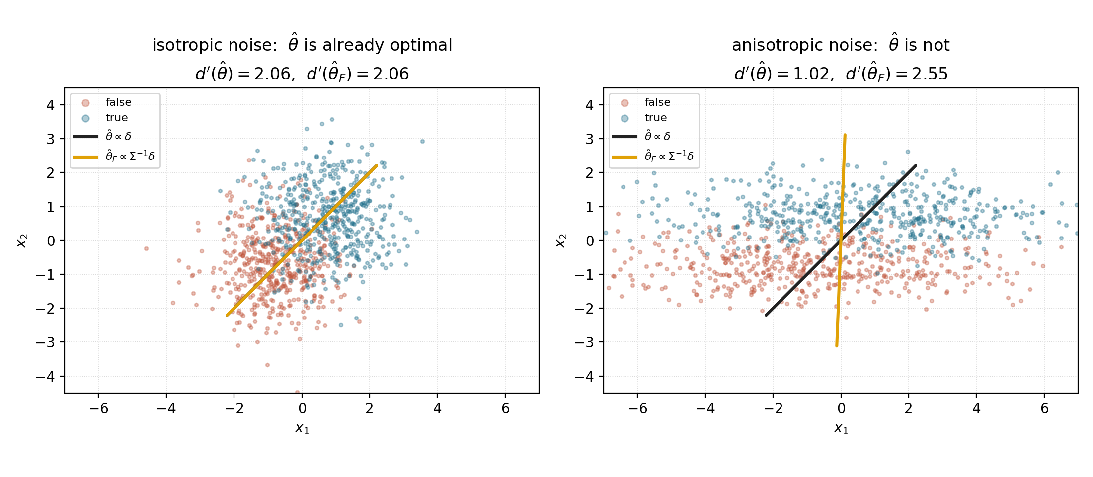
Whitening: the Fisher direction. The mass-mean probe ignores the shape of the within-class noise. If the class-conditional covariance \(\Sigma\) is anisotropic, with large nuisance variance along some directions, the optimal linear discriminant is not \(\mu_1-\mu_0\) but the Fisher/LDA direction

\[\theta_{\mathrm{F}} \;\propto\; \Sigma^{-1}(\mu_1 - \mu_0).\]

This correction is not introduced here. It is the second half of mass-mean probing itself. Marks & Tegmark set \(\theta_{\mathrm{mm}} = \mu_1 - \mu_0\) and then, for IID evaluation, read with \(\sigma(\theta_{\mathrm{mm}}^{\top}\Sigma^{-1}x)\), noting that this coincides with linear discriminant analysis. Their Appendix E gives the same construction in terms of Mahalanobis whitening, and their \(\Sigma\) is the within-class covariance defined exactly as above. What is at issue is where the correction is applied. They are explicit that \(\Sigma^{-1}\) is there to tilt the decision boundary, while \(\theta_{\mathrm{mm}}\) remains the candidate feature direction, one which may be non-orthogonal to that boundary. Their intervention experiments steer along \(\theta_{\mathrm{mm}}\). In their framework, the whitened vector is a readout and the raw mean-difference is the feature. The steering results below report a regime in which that assignment is inverted.

Whitening should raise \(d'\) when the signal is partly buried under structured noise, and hurt when \(n \ll d\) and \(\hat\Sigma\) is ill-conditioned, i.e. where the inverse amplifies estimation error. I estimate \(\Sigma\) with Ledoit–Wolf shrinkage for exactly that regime, and report plain and whitened side by side, since the gap between them is itself diagnostic of how anisotropic the truth geometry is.

The readout framing puts this in familiar company: whitened comparisons of representational geometry have become standard in work on artificial networks (Diedrichsen et al., 2021), and Ying et al. (2026) measure a Mahalanobis cosine between truth probes for exactly the reason above: these representations are anisotropic enough that a raw inner product misleads. A follow-up by Ying, Hase & Kriegeskorte (2026) proves the link between that cosine and readout quality in closed form. For balanced classes with Gaussian projections, a probe’s held-out AUROC is \(\Phi(s/\sqrt{2})\) in its signal-to-noise ratio \(s\), and its Mahalanobis cosine to the Fisher direction is a softsign in the same \(s\). Their \(s\) is the \(d'(u)\) of this post computed with the pooled within-class covariance, and their Fisher distance is \(d'_{\mathrm M}\). One of the conditions under which they show the law fails, a difference-of-means probe far from the Fisher direction, is the regime studied below.

Superposition: the salience knob. Since features share the residual stream, the directions of largest variance need not be the directions of interest. The dominant principal components may encode whatever is most prominent on this dataset (sentence length, topic, token identity) rather than truth. Here a salient direction means a leading principal component of the activations, i.e. one of the directions of largest variance. This is Farquhar’s “most prominent feature” stated geometrically, suggesting a direct test: fit the mass-mean direction after projecting out the top-\(k\) principal components of the activations, taken on the total covariance and so including any between-class shift, and analyze \(d'\) as a function of \(k\). If truth is merely contained in the salient subspace, the signal collapses as soon as the leading components are removed. However, if it occupies its own low-variance subspace, \(d'\) survives. This superposition probe, \(d'\) against the number of top directions removed, is the salience-versus-truth confound turned into a measurement. The measurement itself is reported in The rogue dimension below, once the null is in place.

Drawing a random direction

I build both nulls in this post from random unit vectors. To sample \(u\) uniformly from the unit sphere \(S^{d-1}\), I draw a standard Gaussian and normalize:

\[\xi \sim \mathcal{N}(0, I_d), \qquad u = \frac{\xi}{\lVert \xi \rVert}.\]

This is uniform because the isotropic Gaussian density depends on \(\xi\) only through \(\lVert \xi \rVert\), so it is invariant under every rotation. Normalizing leaves a distribution on the sphere with the same invariance, and the uniform distribution is the only one with that property. (Normalizing each coordinate independently, or sampling coordinates uniformly in \([-1,1]\) and normalizing, does not give a uniform direction, since it concentrates near the cube’s diagonals.)

Two facts about Gaussian random vectors in high dimension enter here. The overlap of such a vector \(u\) with any fixed unit vector \(v\) is small, \(u^{\top} v \sim \mathcal{N}(0, 1/d)\) to a good approximation, so typically \(\lvert u^{\top} v\rvert \approx 1/\sqrt{d}\). Likewise, the overlap with the coordinate axes is \(O(1/\sqrt{d})\). This implies that a random direction is nearly orthogonal to any direction fixed in advance, and by a union bound to every direction on a list at once, so long as the list is not exponentially long in \(d\).

The decoding null. To construct the decoding null, I draw \(u\), compute \(\mathrm{AUROC}(u^{\top}x)\) on held-out data, and fold as above. Repeating this \(n\) times gives the null distribution whose 95th percentile is the \(p_{95}\) of the margin criterion.

A random direction does not achieve \(\mathrm{AUROC} = \tfrac{1}{2}\) merely up to sampling noise. Its projection inherits a share of the real mean shift: \(u^{\top}\delta \sim \mathcal{N}(0, \lVert\delta\rVert^2/d)\), so

\[d'(u) \;\approx\; \frac{\lvert u^{\top}\delta\rvert}{\sqrt{u^{\top}\Sigma u}} .\]

When \(\Sigma\) is close to isotropic, \(u^{\top}\Sigma u \approx \operatorname{tr}\Sigma / d\) and the factors of \(d\) cancel, leaving \(d'(u) \approx \lvert z \rvert \cdot \lVert\delta\rVert / \sqrt{\operatorname{tr}\Sigma}\) with \(z \sim \mathcal{N}(0,1)\). The null is therefore large exactly when the true separation is large. It is not a fixed background, and it must be recomputed for every layer and dataset.

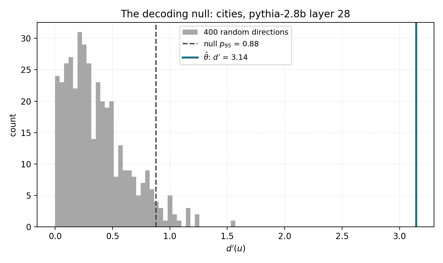
The steering null. A steering direction \(w\) is added to the activation rather than projected onto it. I draw \(w\) the same way, add it to the residual stream, and measure how the model’s behavior moves: this measures what an arbitrary direction causes, rather than what it reads. A direction can clear the decoding null without clearing the steering null or vice versa. Throughout this post an effect, decoding or steering, is called significant when it clears the 95th percentile of its null, and the word is used in no other sense.

The scale of an intervention

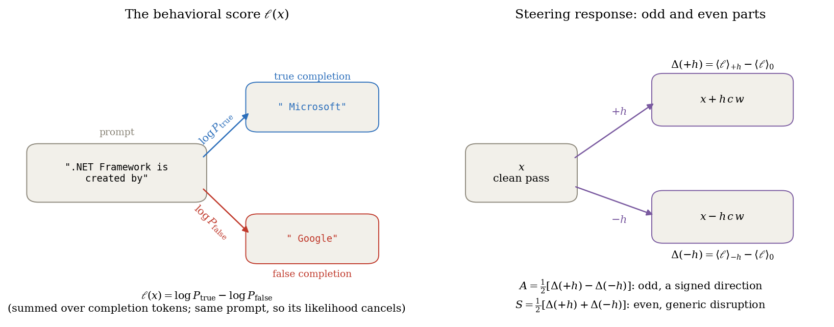
The behavioral score. What steering moves is the model’s preference between two completions of the same prompt. Each statement is split at its final entity into a prompt and a pair of one-entity completions. On cities the prompt is “The city of Krasnodar is in” with true completion “ Russia” against a paired false country. On counterfact, the shipped relation template, e.g. “.NET Framework is created by” with “ Microsoft” against “ Google”. The score is

\[\ell(x) \;=\; \log P(\text{true completion} \mid \text{prompt}) \;-\; \log P(\text{false completion} \mid \text{prompt}),\]

summed over the completion’s tokens. Both completions are scored against the same prompt, so the prompt’s own likelihood cancels and only the preference between the two entities remains.

Steering displaces the residual stream, \(x \mapsto x + h\, c\, w\). The unit \(c\) sets the scale, and should be chosen so that the effects of interest appear at \(h \sim 1\). Much smaller displacements cannot move a statement across the decision boundary, and much larger ones push the activation far outside the range the model ever sees, where the response is large, idiosyncratic, and mostly independent of which direction was pushed. The steering null widens sharply in that regime, which is a useful diagnostic in its own right. If a random direction of the same length produces as much behavioral change as the chosen direction, \(h\) is too large.

Taking \(c = \sigma_w = \operatorname{std}(w^{\top} x)\), the spread of activations along \(w\), seems natural but is a trap: \(\sigma_w\) depends on the direction, so different conditions of an experiment receive pushes of different magnitude. It also depends on the layer, so a fixed \(h\) means different things at different depths.

The right unit is the class-mean gap \(c = \lVert\hat\delta\rVert\), which is a property of the dataset and layer rather than of the direction. Then \(h = 1\) displaces an activation by exactly the distance between the two class means, so that along \(\hat\theta\) it carries the false-class centroid onto the true-class centroid. Every displacement is norm-matched and each layer is comparable.

Decomposition. The shift in \(\ell\) at coefficient \(h\), averaged over the evaluation set, is \(\Delta(h) = \big\langle\, \ell(x + h\, c\, w) - \ell(x) \,\big\rangle\). I express the symmetric and antisymmetric parts of the shift as:

\[A \;=\; \tfrac{1}{2}\big[\Delta(+h) - \Delta(-h)\big], \qquad S \;=\; \tfrac{1}{2}\big[\Delta(+h) + \Delta(-h)\big].\]

Only the antisymmetric part \(A\) is evidence of a direction: pushing along \(\hat\theta\) should make the model favor the true completion and pushing against it the false one, so a genuine truth direction responds as an odd function of \(h\). A generic perturbation degrades the computation whichever way it points, contributing to \(S\) and leaving \(A\) near zero.

Seeds and draws. I define a seed as a resampling of the class-stratified train/test split. Averaging over seeds gives the standard error on the given direction’s effect, that is, the reproducibility of the measurement. I define a draw as a resampling of a fresh random direction (\(u\) for a decoding null, \(w\) for a steering null). Since no fitting is involved, the drawn direction does not depend on the split, and the draws simply provide the null distribution. A tight seed error bar says nothing about whether the effect sits inside the null.

Setup

Models. I use the Pythia suite (Biderman et al., 2023) at 70m, 410m, 1.4b, and 2.8b parameters. They share architecture, data and training order and differ only in scale, which is what makes it the right ladder for an emergence question. Residual widths are \(d = 512, 1024, 2048, 2560\).

Data. I use the twelve curated true/false sets from Marks & Tegmark. Nine form a main tier, cities, neg_cities, larger_than, smaller_than, cities_cities_conj, cities_cities_disj, common_claim_true_false, companies_true_false and counterfact_true_false, subsampled class-balanced to \(N = 1198\), the size of the smallest member rounded to a class-balanced count, so that \(d'\), transfer, and the ratio \(N/2d\) are directly comparable across datasets. Two translation sets (sp_en_trans, neg_sp_en_trans) have only \(N = 354\) and are reported separately. The likely set is included as a distractor: it is constructed so that textual plausibility decorrelates from truth, so a direction fitted on it isolates the plausibility axis on its own. These datasets, the papers that introduced them, and their known failure modes are catalogued in a companion map of the truth-probing literature.

Activations. I pass each statement through the model once, and the residual stream is read at the final real token (right-padded, located from the attention mask) at every layer. Layer \(0\) is the embedding, before any transformer block. On templated statements the last-token embedding is nearly constant within a dataset, so its \(d'\) is degenerate and it is excluded from layer selection.

Estimation, held out. I fit every quantity on a class-stratified training half and evaluate on the held-out half: the mass-mean direction, the within-class covariance used for whitening, and the PCA basis used by the superposition probe. The estimator is not prone to overfitting in the usual sense, since it has almost no capacity, fitting only two class means. However, with \(d\) comparable to \(N\) the estimated mean difference absorbs \(O(\sqrt{d/N})\) of noise, and scoring it in-sample biases \(d'\) upward through exactly the fluctuations that defined the direction. In practice the correction is large. On a synthetic control with isotropic noise, a planted separation of \(d' = 1\), and the post’s own \(d = 2560\) and \(N = 1198\), the in-sample estimate returns \(4.2\) and the held-out estimate \(0.24\). Both follow from the derivation in How small is too small?: the noise in \(\hat\theta\) is aligned with the sample fluctuations that produced it, so in-sample \(d'^{2} \simeq 1 + 4d/N_{\text{train}}\), while held-out \(d' \simeq \cos(\hat\theta, \theta) \simeq (1 + 4d/N_{\text{train}})^{-1/2}\). The simulation matches the in-sample prediction to within \(2\%\) and the overlap \(\cos(\hat\theta, \theta)\) to within \(4\%\) for \(d/N_{\text{train}}\) from \(0.2\) to \(14\). The held-out \(d'\) itself scatters more, \(-11\%\) to \(+16\%\) about its prediction, because it is estimated on a finite held-out half: its standard deviation across repetitions is about \(0.08\), so a twenty-repetition mean is fixed only to about \(\pm 0.02\), and every deviation sits within two of those.

Two consequences follow. First, the held-out \(d'\) is attenuated: the fitted \(\hat\theta\) is misaligned with the true direction by \(O(\sqrt{d/N_{\text{train}}})\), so the reported \(d'\) underestimates the intrinsic separation on average, and the attenuation is largest for the widest model. Second, \(d'\) is sign-blind while AUROC is not, so \(\hat\theta\) is oriented on the training half and that sign is held fixed on the test half. Layer selection then maximizes held-out AUROC above the layer’s own null, which cannot reward an anti-predictive direction. Selecting a layer by an SNR is itself the field’s practice. Bürger et al. take the layer maximizing the ratio of between- to within-class variance, and later work adopts the recipe unchanged (Bao et al. select the layer for every model in their study by that ratio, crediting Bürger et al. and MacDiarmid et al. for the technique. Poulis et al. App. B.1 write out the form Bürger and Bao are using, a ratio of squared mean differences to variances averaged across dimensions). That is \(d'^{2}\) averaged over coordinates, with no direction and no null defined. The margin used here is the same ratio along one direction, read against what random directions give.

The null. At every layer I draw \(200\) random unit directions for the decoding null, evaluate them on the same held-out points, and fold as above. The null is recomputed per layer rather than once globally: where the class gap grows with depth relative to the total spread, a random direction inherits more of it, and the null rises with the signal it is meant to calibrate.

Whitening. \(\hat\Sigma_{\text{LW}}\) as defined above. At \(N_{\text{train}} \approx 600\) against \(d = 2560\) the shrinkage is what makes the inverse usable.

Where the direction is recoverable

With the null, \(d'\), and the class-mean-gap unit in place, the reproduction question becomes concrete: at what scale, at what depth, and across which datasets is a truth direction actually recoverable?

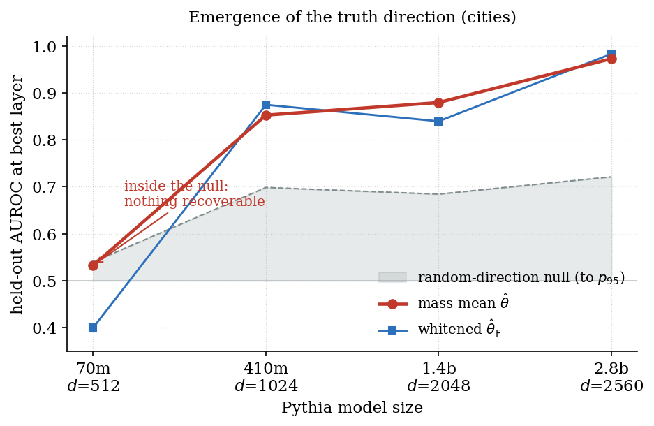
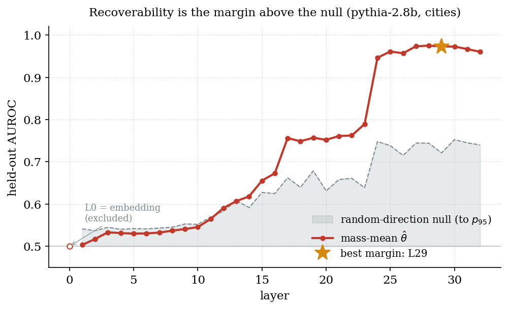
Across the Pythia ladder it emerges with scale. On cities the best-layer mass-mean AUROC climbs from \(0.53\) at pythia-70m, inside the random-direction null (\(p_{95} = 0.54\)) and so not recoverable, to \(0.85\) at 410m, \(0.88\) at 1.4b, and \(0.97\) at 2.8b, with \(d'\) rising from \(0.07\) to \(2.93\). At 70m the whitened direction does not clear the null at any layer either, the best value being \(0.504\) on cities and \(0.520\) on counterfact. What fails there is the whole linear class, not one estimator within it. Whether a 70m model represents truth in some form this class cannot express is not tested here.

Within a single model, the truth direction is a property of depth. Sweeping the layers of pythia-2.8b on cities, the mass-mean AUROC sits inside the null through the early layers, lifts clear of it around the middle of the network, and plateaus high across the late layers, peaking at \(0.975\) at layer \(28\). The null itself widens with depth, its 95th percentile climbing from \(0.54\) early to \(0.75\) deep, so recoverability is again the margin above the null, not the raw number: a deep-layer AUROC in the low \(0.7\)s can still sit inside it. Layer selection maximizes the margin, not the AUROC, and the two peak one layer apart: the AUROC at layer \(28\) (\(0.975\) against a null of \(0.744\)), the margin at layer \(29\) (\(0.973\) against \(0.721\)). The scale ladder above reports layer \(29\), since the margin is what carries the claim.

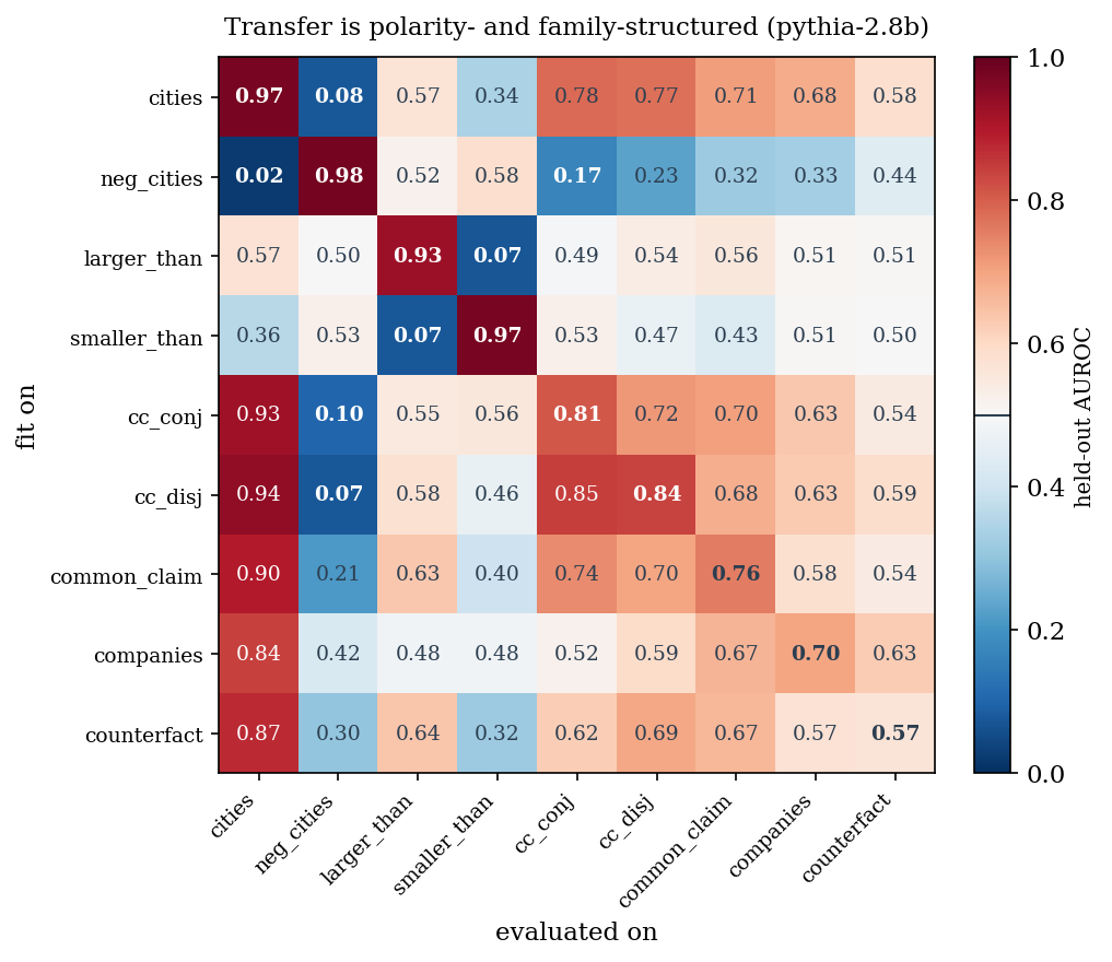
The direction transfers, but only within a polarity and a family. Fitting the mass-mean direction on one main-tier set and evaluating it on another reproduces the within-dataset signal on the diagonal, \(0.93\) to \(0.98\) for the single-frame sets and down to \(0.57\) for counterfact, but the off-diagonal is organized, not merely weak. Three structures are visible in the full nine-by-nine matrix. First, between a statement type and its logical negation the transfer is anti-predictive: cities scores AUROC \(0.08\) on neg_cities and larger_than scores \(0.07\) on smaller_than, both far below chance, so the same vector reads truth backwards once polarity flips. The neg_cities direction is anti-predictive not on cities alone but on the compound and claim-like sets as well, \(0.02\) to \(0.33\) across five of them. Second, the sets fall into two families that do not speak to each other. The numeric comparisons transfer to nothing outside their own pair, \(0.32\) to \(0.64\) in both directions, while cities, the two compound sets, common_claim, companies and counterfact form a block that transfers within itself at \(0.52\) to \(0.94\). Third, that block is asymmetric, and the asymmetry belongs to the receiver rather than to the direction. The cities column is uniformly high, \(0.84\) to \(0.94\) from every other member, because a transferred score is \(\Phi(d'/\sqrt2)\) with the target’s gap and noise inside \(d'\), and cities has the largest gap in the benchmark. A direction that reads its own set at \(0.57\) still reads cities at \(0.87\). Transfer AUROC scores the receiver’s signal-to-noise as much as the direction’s alignment, so the matrix has to be read by rows and columns together. The mass-mean direction is genuinely there, but a single vector approximates a structure carrying at least a separate polarity axis and a family axis. The below-chance cells are what the decomposition of Bürger et al. (2024) predicts: a direction fit on affirmative statements alone is a mixture \(t_A = \alpha\, t_G + \beta\, t_P\) of a general truth direction and a polarity-sensitive one that reads truth forwards on affirmatives and backwards on negations, so under negation the \(t_P\) term anti-correlates with the label, and an AUROC of \(0.08\) rather than \(\tfrac{1}{2}\) says that term dominates the mixture at this layer. The comparison is direct, not analogical: their cities/neg_cities pair is the Marks & Tegmark pair used here. Poulis et al. (2026) measure the same signature in Llama, affirmative-trained probes anti-predictive on negations (AUROC \(\approx 0\)) at the depths where the polarity direction carries most of the truth-related variance.

The sweep covers all twelve sets, not only the nine of the transfer matrix. Every templated set with a single frame clears its null comfortably (plain AUROC \(0.93\)–\(0.98\) at its selected layer). The two free-form sets sit at the bottom of the table (\(d'_{\mathrm{mm}} = 0.64\) and \(0.20\)). companies_true_false shows the largest plain/whitened gap in the benchmark, a second instance of the rogue-dimension pattern, decoded rather than steered. The full table and per-dataset commentary are in the appendix Results on the full twelve-dataset benchmark.

The plausibility axis has the opposite depth profile. The likely set carries no truth labels at all. Its two classes are the most likely and hundredth-most-likely final token, so a direction fitted on it reads textual probability alone. This axis is easy to find. On pythia-2.8b the mass-mean direction reaches held-out \(\mathrm{AUROC} = 0.890\) (\(d'_{\mathrm{mm}} = 1.75\)) at layer \(12\), against a null 95th percentile of \(0.593\), a wider margin than counterfact achieves at any depth. What separates it from the truth sets is the depth at which it is recoverable. Plausibility is already readable in the embedding (\(0.700\) at layer \(0\)), peaks at layers \(11\) and \(12\) (the AUROC at \(11\), the margin at \(12\)), and then decays through the second half of the network to \(0.657\) by layer \(28\). cities runs the other way: inside the null through the early layers, clear of it by mid-network, peaking at \(0.973\) at layer \(29\). In one model, the direction that reads probability and the direction that reads truth are strongest at opposite ends of the depth axis, which is a reason to doubt that the deep-layer truth direction is plausibility in disguise.

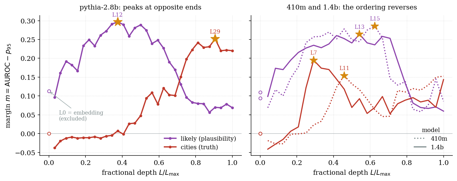
One limit on that reading, and one further test, should be stated. The limit is that the profiles are cleanest at 2.8b. At 410m and 1.4b the plausibility peak stays mid-network (\(L = 15\) and \(L = 13\) of \(24\)) but cities peaks earlier rather than later (\(L = 11\) and \(L = 7\)), so the ordering is reversed, and the late-depth structure survives only as a secondary rise over the final layers (\(m = 0.153\) at 410m layer \(24\), \(0.144\) at 1.4b layer \(24\), the last block at both widths, where the margin is still rising). The test is the one Marks & Tegmark designed the set for, the cross-dataset one: take a direction fitted on truth statements and evaluate it on likely. A direction that had been reading plausibility all along should separate it. However, none of them do. Across all nine main-tier sets, a direction fitted at that set’s own selected layer and evaluated on held-out likely gives AUROC between \(0.44\) and \(0.60\), and not one clears the random-direction null on likely at the corresponding layer (\(p_{95} \approx 0.58\)–\(0.60\)). The largest is larger_than at \(0.598\) against a null of \(0.600\). cities gives \(0.559\) and counterfact \(0.480\). The reverse direction agrees: the likely-fitted direction scores \(0.43\)–\(0.54\) on the nine truth sets. So the plausibility axis and the truth directions are separately readable and mutually uninformative. This is what the distractor was constructed to detect, and it comes out clean.

How small is too small?

Cover’s theorem marks \(2d\) as the scale below which separability stops being informative. The shuffled-label control measures what that costs in practice: fit the mass-mean direction to a random permutation of the labels and record how much separation comes back.

The control is the control task of Hewitt & Liang (2019), and the gap between real-task and control-task performance is what they call selectivity. Their diagnosis and their prescription concern probe capacity: a probe expressive enough to memorize the control task is too expressive to trust, so a smaller one should be used. That prescription has no purchase here. The mass-mean probe fits two class means and nothing else, and on counterfact at \(N = 100\) it still separates shuffled labels with AUROC \(0.80\) on pythia-2.8b (\(0.795 \pm 0.042\) over sixteen permutations), which is what the true labels reach in sample at the same \(N\). There is no capacity to shrink. The freedom is in the ambient dimension.

This control is the one place in the post where a direction is scored on the points it was fitted to. Everywhere else a direction is fitted on a training split and scored held-out. Here that would defeat the purpose, since on held-out data a shuffled-label direction scores \(\tfrac{1}{2}\) by construction, and the quantity of interest is exactly how much separation the estimator manufactures from the noise it was fitted to. Scoring in sample is what exposes it. Pooling the four models, the excess AUROC a mass-mean direction extracts from pure noise scales as

\[\mathrm{AUROC}_{\text{shuffled}} - \tfrac{1}{2} \;\approx\; 0.045 \left(\frac{N}{2d}\right)^{-0.49}.\]

The exponent follows from the estimator alone. \(\hat\theta\) is a difference of two sample means, each concentrating at the \(\sqrt{N}\) rate, so the noise it carries has magnitude \(O(\sqrt{d/N})\) whatever the activations look like, and the excess must fall as \(N^{-1/2}\) at fixed \(d\). Measured across four models and \(N\) from \(100\) to \(32{,}000\), it comes back \(-0.49\). The phenomenon is dimensional slack, the room that \(d \gg N\) leaves for a direction built from a sample’s own fluctuations to separate that sample, since the fluctuations that define the direction are the ones being scored. It is not capacity.

Inverting the law gives the condition for noise alone to contribute less than \(\varepsilon\) of excess AUROC,

\[N \;>\; 2d\left(\frac{a}{\varepsilon}\right)^{1/\lvert b\rvert} \;=\; 2d\left(\frac{0.045}{\varepsilon}\right)^{2.0} ,\]

which at the widths in this post and the standard 7B width gives the following. The table uses the unrounded fit, \(a = 0.0446\) and \(b = -0.487\), and the rounded values reproduce each entry to within about \(2\%\).

\(d_{\text{model}}\)	\(N\) for \(\varepsilon = 0.05\)	\(\varepsilon = 0.02\)	\(\varepsilon = 0.01\)
\(512\)	\(809\)	\(5{,}305\)	\(22{,}024\)
\(2{,}048\)	\(3{,}233\)	\(21{,}220\)	\(88{,}093\)
\(2{,}560\)	\(4{,}041\)	\(26{,}525\)	\(110{,}117\)
\(4{,}096\)	\(6{,}465\)	\(42{,}440\)	\(176{,}186\)
\(8{,}192\)	\(12{,}930\)	\(84{,}879\)	\(352{,}372\)

The curated true/false datasets in this literature hold \(N \approx 1{,}200\) statements. For a \(d = 4096\) model, the width of the 7B models these probes are usually run on, noise alone buys in-sample AUROC \(0.55\) until \(N \approx 6{,}500\) and \(0.52\) until \(N \approx 42{,}000\). Every dataset in the benchmark is between five and thirty times too small for an in-sample AUROC in the seventies to mean what it appears to mean. Held-out scoring removes the inflation but not its source. The fitted direction is the same object either way, and at these sizes it is mostly noise: the synthetic control in Setup puts its overlap with the true direction at \(0.24\) for the post’s own \(d/N_{\text{train}}\). Held-out evaluation reports that attenuated direction’s honest score, which is why held-out \(d'\) errs low where in-sample \(d'\) errs high.

The newest state-of-the-art lie detector sits deeper still in this regime. The topic datasets of Bürger et al. run from \(N = 164\) (animal_class) to \(1{,}496\) (cities) at \(d = 4096\), so \(N/2d\) falls between \(0.02\) and \(0.18\). Their leave-one-topic-out protocol is held-out, which is the right defense, and the table says how much it defends against: at these sizes the slack is available in full to anything fit or diagnosed in sample.

The control also behaves correctly at the other end of the ladder. On pythia-70m the true and shuffled curves lie on top of each other at every \(N\), which is what a model with nothing recoverable in it should give: on this dataset neither the plain nor the whitened direction clears the random-direction null at any layer, so there is no signal for the true labels to add.

The prefactor is where the dataset enters. What it quantifies is the number of directions the noise effectively occupies. A spectrum concentrated on a few axes leaves a random labeling less room to find a separator than a flat one does, so the ambient width \(d\) is the right count only when the spectrum is flat. In general the count is the participation ratio of the within-class covariance, and the amplitude should collapse across datasets once \(N\) is measured in units of it.

A second sweep tests the exponent and the prefactor across datasets. The control is scored in sample, so no half has to be held back and the grid can run to the full set. Repeating it on pythia-2.8b at each dataset’s own best layer, over a seven-point geometric grid from \(N = 100\) to that dataset’s total with sixteen label permutations per point, and fitting \(\mathrm{AUROC}_{\text{shuffled}} - \tfrac{1}{2} \approx a\,(N/2d)^{b}\) on each, gives

dataset	\(N_{\max}\)	\(a\)	\(b\)	\(R^{2}\)	\(\mathrm{PR}\)	\(\hat\lambda_1/\operatorname{tr}\hat C\)
counterfact_true_false	\(3000\)	\(0.045\)	\(-0.490 \pm 0.019\)	\(0.993\)	\(30.3\)	\(0.11\)
cities	\(1496\)	\(0.053\)	\(-0.446 \pm 0.009\)	\(0.998\)	\(34.6\)	\(0.11\)
larger_than	\(1980\)	\(0.027\)	\(-0.484 \pm 0.014\)	\(0.996\)	\(8.9\)	\(0.28\)
sp_en_trans	\(354\)	\(0.064\)	\(-0.413 \pm 0.044\)	\(0.947\)	\(16.8\)	\(0.23\)

The exponents look scattered, and taken at face value cities sits six standard errors from \(-\tfrac12\). They are scattered not by dataset but by how far up in \(N\) each grid reaches, because the power law is asymptotic and its small-\(N\) end is shallower than \(-\tfrac12\). Refitting counterfact over truncated windows makes this explicit:

\[b = -0.385 \pm 0.029 \;\; (N \le 400), \qquad -0.445 \pm 0.019 \;\; (N \le 1500), \qquad -0.490 \pm 0.019 \;\; (\text{all } N).\]

Each of the other three then matches counterfact restricted to its own reach. cities stops at \(1496\) and gives \(-0.446\) against \(-0.445\), larger_than reaches \(1980\) and gives \(-0.484\) against \(-0.465\), and sp_en_trans stops at \(354\) and gives \(-0.413\) against \(-0.385\), within its own error. With the fitting window matched the four agree, so the dataset-independence of the exponent is measured rather than only argued from the estimator, and the best estimate of the asymptotic value is the one with the longest lever arm, \(-0.490 \pm 0.019\) over \(1.5\) decades. That is the predicted \(N^{-1/2}\) to within half a standard error, and both it and its amplitude \(0.045\) reproduce the pooled four-model fit above.

For the amplitude, \(a\) is the wrong statistic to compare across datasets, since each \(a\) is defined at its own fitted \(b\). It is also not a free parameter. Under shuffled labels there is no signal, so within a class \(x \sim \mathcal{N}(0, \Sigma)\), and the mass-mean direction is a signed sum of the samples,

\[\hat\theta \;=\; \hat\mu_{+} - \hat\mu_{-} \;=\; \frac{2}{N}\sum_i \epsilon_i x_i , \qquad \epsilon_i = \pm 1 ,\]

so \(\hat\theta \sim \mathcal{N}\!\left(0, \tfrac{4}{N}\Sigma\right)\) and

\[\mathbb{E}\lVert\hat\theta\rVert^{2} = \frac{4}{N}\operatorname{tr}\Sigma , \qquad \mathbb{E}\,\hat\theta^{\top}\Sigma\,\hat\theta = \frac{4}{N}\operatorname{tr}\Sigma^{2} .\]

The in-sample separation it produces is the projected class gap, which is its own squared length, over the projected within-class spread,

\[d'_{\text{in}} \;=\; \frac{\lVert\hat\theta\rVert^{2}}{\sqrt{\hat\theta^{\top}\Sigma\hat\theta}} \;\simeq\; \frac{2}{\sqrt{N}}\,\frac{\operatorname{tr}\Sigma}{\sqrt{\operatorname{tr}\Sigma^{2}}} \;=\; 2\sqrt{\frac{\mathrm{PR}}{N}} ,\]

which is where the participation ratio enters: \(\mathrm{PR} = (\operatorname{tr}\Sigma)^{2}/\operatorname{tr}\Sigma^{2}\) is the count of directions the noise occupies, and it equals \(d\) only for a flat spectrum. With \(\mathrm{AUROC} = \Phi(d'/\sqrt{2})\) and \(\Phi(x) \simeq \tfrac12 + x/\sqrt{2\pi}\) at small argument,

\[\mathrm{AUROC}_{\text{shuffled}} - \tfrac{1}{2} \;\simeq\; \frac{d'_{\text{in}}}{2\sqrt{\pi}} \;=\; \frac{1}{\sqrt{\pi}}\sqrt{\frac{\mathrm{PR}}{N}} ,\]

so the collapse constant is predicted rather than fitted:

\[C \;\equiv\; \Bigl(\mathrm{AUROC}_{\text{shuffled}} - \tfrac{1}{2}\Bigr)\sqrt{\frac{N}{\mathrm{PR}}} \;=\; \frac{1}{\sqrt{\pi}} \;=\; 0.564 .\]

Measured, \(C\) is flat to about \(\pm 10\%\) within a dataset over a thirtyfold range in \(N\), and runs from \(0.51\) to \(0.65\) across counterfact, cities and larger_than, against a factor \(2.0\) in \(a\) and \(3.9\) in \(\mathrm{PR}\). The dependence on the spectrum runs the way the count predicts and against the intuitive direction: larger_than is the most concentrated set, \(\mathrm{PR} = 8.9\) with \(28\%\) of the within-class variance on one axis, and it carries the smallest amplitude of the three.

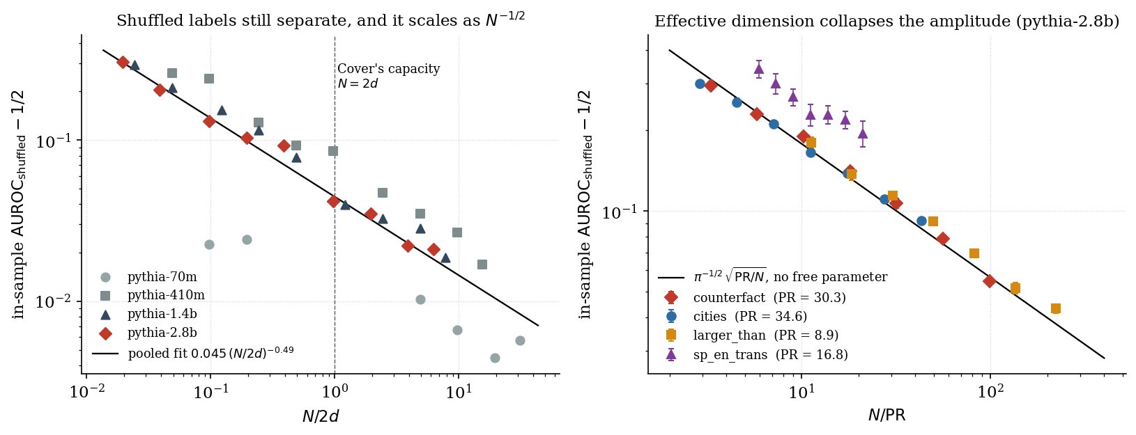
sp_en_trans does not join the collapse. It sits at \(C = 0.77\) to \(0.90\), well above \(1/\sqrt{\pi}\), where the other three bracket it. The derivation factors into two independent steps, and measuring them separately localizes the miss. The distributional step holds: \(\mathrm{AUROC}\) tracks \(\Phi(d'_{\text{in}}/\sqrt{2})\) to within \(3\%\) on all four datasets, this one included, despite its projections carrying the largest excess kurtosis of the four (\(+0.8\) to \(+1.2\) against \(-0.7\) to \(+0.2\) elsewhere). The discrepancy is in the second-moment step: the measured \(d'_{\text{in}}\) runs \(1.47\) to \(1.62\) times \(2\sqrt{\mathrm{PR}/N}\) here, against \(1.03\) to \(1.17\) on the other three.

Two explanations were tested which both fail. Near-duplicate items would inflate an in-sample fit by making the effective sample smaller than \(N\). However, sp_en_trans has \(344\) distinct Spanish words across its \(354\) statements, while cities has exactly two statements per subject and collapses normally. Under-measurement of \(\mathrm{PR}\) is the other candidate, since \(\mathrm{PR}\) is itself a sample quantity that rises without saturating below \(N \approx 1000\), and sp_en_trans can only be read at \(N = 354\). But restricting each of the other three to a pool of \(354\) statements and re-reading \(\mathrm{PR}\) from that pool leaves them between \(1.08\) and \(1.15\), nowhere near \(1.5\). The anomaly is a property of sp_en_trans rather than of its size. It sits in the second-moment step rather than in the shape of the projection, and it is not explained here.

The sweep varies the dataset at fixed model and identifies the quantity that sets the prefactor at a given width. It does not test whether \(\mathrm{PR}\) should replace \(2d\) across the scale ladder, where the two co-vary, and the pythia-70m points below the pooled line in the figure are that question in its across-model form. The inversion table therefore remains a guide at the ambient width, read upward for a dataset whose within-class noise is spread out and downward for one whose noise is concentrated.

A steering effect with the wrong sign

The decoding analysis says when a truth direction is readable. Steering asks the separate question of whether it is causal, that is, whether displacing the residual stream along \(\hat\theta\) moves the model’s behavior toward the true completion. The two need not agree. On counterfact_true_false at the deep layers of pythia-2.8b the mass-mean direction is neither readable nor correctly causal. For the readout, the held-out AUROC at layer \(28\) is \(0.502\) against a null of \(0.560\), and it stays inside the null at every layer except for the last. As an intervention it produces a significant effect with the wrong sign.

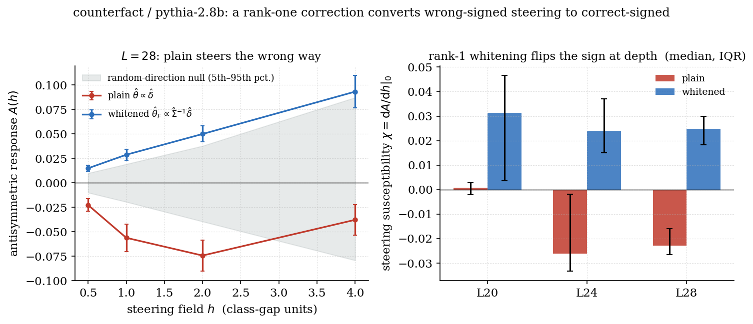
As defined above, steering is reported as the antisymmetric response \(A\) in class-gap units. A genuine truth direction produces \(A > 0\), and the random-direction steering null fixes the bar \(A\) must clear. Across ten seeds at layer \(28\), at a displacement of one class gap, the mass-mean direction returns

\[A(1) < 0 \;\text{ in } 8/10 \text{ seeds, each at } p \le 0.003, \qquad \operatorname{med}_{\text{seeds}} A(1) = -0.062, \qquad \sigma_{\text{null}} = 0.012,\]

where \(p\) is the fraction of the \(400\)-draw random-direction null of \(A(1)\) at least as extreme in the same direction, evaluated seed by seed. The seed median sits five null standard deviations below zero, and the two positive seeds sit inside the null. The linear steering susceptibility \(\chi\), the through-origin slope of \(A\) against \(h\) over \(h \le 4\), is \(-0.023\) at this layer. It is a diluted summary of the same effect. The response is not linear in \(h\), and by \(h = 4\), four class gaps out, \(A\) has already fallen back toward zero, which is the regime The scale of an intervention warned about. Layer \(24\) gives the same sign less cleanly: \(7/10\) seeds negative with a median \(A(1) = -0.037\) against a null standard deviation of \(0.015\), and one seed strongly positive. The effect is not null. It is significantly wrong-signed. Displacing an activation toward the true-class centroid, along the very vector the estimator returns for truth, makes the model measurably less likely to produce the true completion.

Because \(\hat\theta\) reads at chance here, that significance carries the whole claim. A direction sitting inside its decoding null is expected to do nothing under intervention, and a small negative point estimate on its own would not be distinguishable from noise. What makes this a result rather than a null is that the effect clears a \(400\)-draw random-direction null in the wrong direction, reproducibly across seeds and at two layers.

The slope of behavioral response against steering coefficient is not a new summary. It is the steerability of Tan et al. (2024), who fit exactly this line through a logit-difference propensity curve. Their intervention displaces the last token position only, where the harness here displaces every position, so magnitudes are not directly comparable across the two. What is added here is the split into even and odd parts, so that degradation and signed effect are separated, and the random-direction null that says which susceptibilities are distinguishable from chance.

Read naively, this is a failure of the linear picture. Displacing along the direction fit to read truth does not raise the probability of the true completion. It lowers it. That reading would put counterfact in the column of cases where the truth direction is an artifact of the readout, epiphenomenal to the behavior. It does not even earn that description. At this depth \(\hat\theta\) sits inside its decoding null, so there is no separation for the steering result to be epiphenomenal to. However, I use the rest of this post to argue that the naive reading is wrong: the wrong sign is a property of the estimator, not of the activation geometry. What that means precisely is that the same activations, at the same layer, contain a direction along which displacement moves the model toward the true completion. But the mass-mean rule does not return that direction. It returns \(\hat v_1\), the axis of largest within-class variance, with which \(\hat\theta\) shares a cosine of \(0.994\) at this depth. The weight of that claim rests on the correction rather than on a mechanism for the wrong sign: replacing the mass-mean rule by the Fisher rule, inside the same linear class, recovers the correct sign, while what makes the plain direction negative at layer \(28\) turns out to lie beyond first order and is not settled here. Change the rule, either by downweighting that axis or by deleting it outright, and the correct sign comes back out of the same data. The claim is about which part of the geometry the estimator points at, not about how much truth the layer encodes. How well the corrected direction reads is a separate question, quantified in the next section by its held-out AUROC against the decoding null.

The rogue dimension

Definition. I call \(\hat v_1\) a rogue dimension when it dominates the within-class covariance, that is, \(\hat\lambda_1/\operatorname{tr}\hat C \approx 1\) or equivalently \(\mathrm{PR} \approx 1\) and \(\hat\lambda_1/\hat\lambda_2 \gg 1\). This condition is a statement about the noise geometry alone and is basis-free and independent of any probe. The estimator only becomes involved through the separate question of whether \(\hat\theta\) has aligned with it.

This is deliberately not the same object as the massive activations of Sun et al., which are individual coordinates whose magnitude far exceeds the median, nor the rogue dimensions of Timkey & van Schijndel, which are coordinates that dominate cosine similarity. Those are properties of the mean and of a basis. This is a property of the covariance and of no particular basis. The distinction is important here. At counterfact layer \(8\) the two coincide: \(\hat v_1\) carries \(86\%\) of its mass on a single coordinate, and that coordinate’s mean activation is \(1446\times\) the median across coordinates, a massive activation by their criterion. By layer \(28\) the eigenvector has delocalized, \(37\%\) on its largest coordinate and \(90\%\) across five, so the rogue dimension is no longer any one neuron. cities at layer \(28\) still has the massive activation, the same coordinate at \(563\times\) the median, and has no rogue dimension at all. Its leading eigenvector holds half a percent of its mass on any coordinate. A massive activation is nearly constant across statements, so it inflates the mean without inflating the within-class covariance. It produces a rogue dimension only when the remaining variance is small enough for it to dominate.

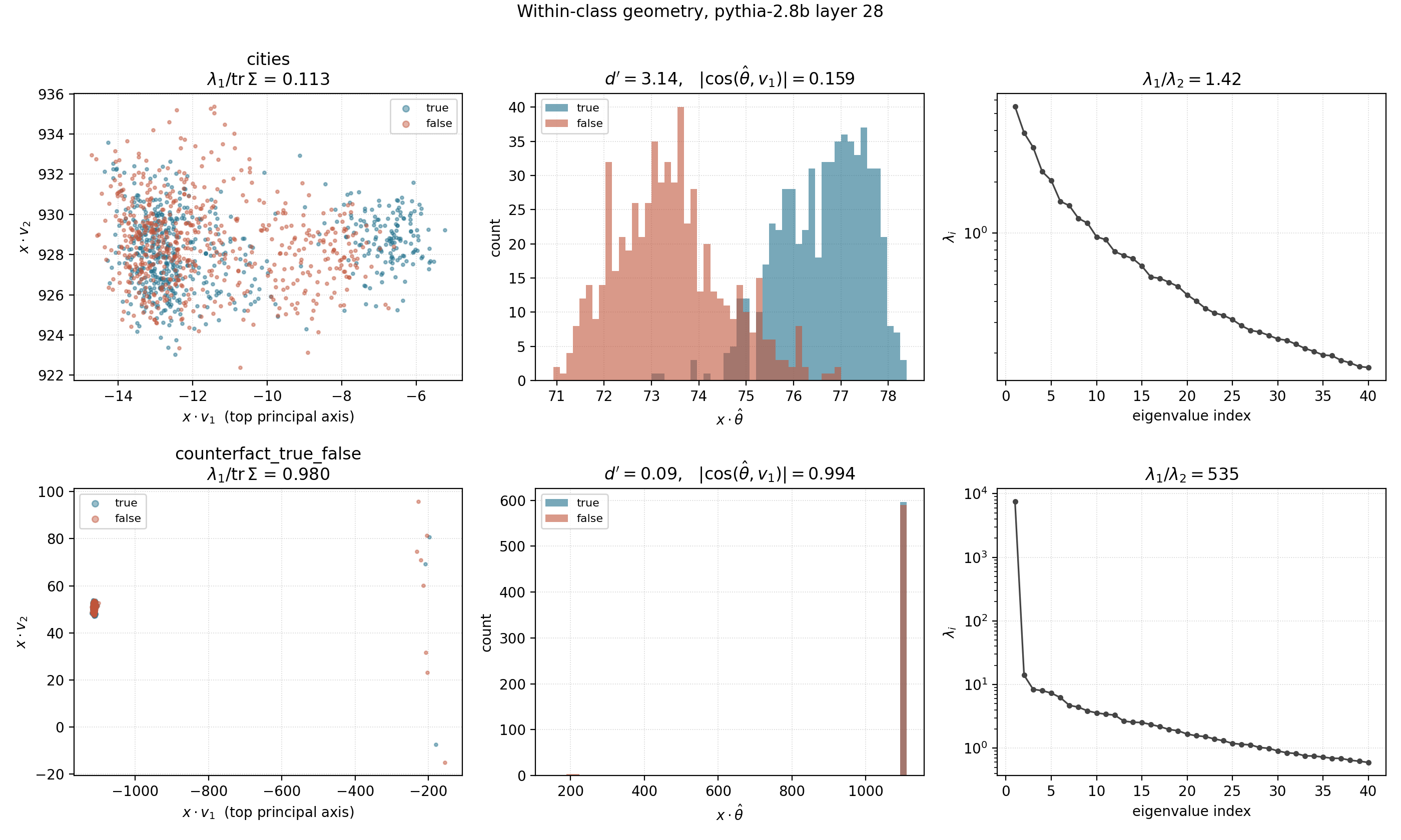
The diagnosis is in the spectrum of the within-class covariance. I diagonalize \(\hat C = \sum_i \hat\lambda_i \hat v_i \hat v_i^{\top}\) with sample eigenvalues \(\hat\lambda_1 \ge \hat\lambda_2 \ge \dots\) and eigenvectors \(\hat v_i\), and measure where the mass-mean direction sits relative to its leading eigenvector. On counterfact at pythia-2.8b, layer \(28\):

\[\frac{\hat\lambda_1}{\operatorname{tr}\hat C} = 0.980, \qquad \frac{\hat\lambda_1}{\hat\lambda_2} = 535, \qquad \lvert\cos(\hat\theta, \hat v_1)\rvert = 0.994 .\]

A single eigendirection carries \(98\%\) of the within-class variance. It is \(535\) times larger than the next, and the mass-mean direction is almost perfectly aligned with it. Therefore, the estimator has not returned a truth direction, it has returned \(\hat v_1\), the dominant axis of the within-class noise. On this dataset there is essentially no class-gap signal for \(\hat\delta\) to lock onto, so the finite-sample \(\hat\delta\) is dominated by its projection onto the highest-variance axis. This axis is the salient direction of the superposition test above. When the class gap is negligible, the leading direction of the total activation covariance and the within-class \(\hat v_1\) coincide, so the two diagnostics see the same axis. They separate only once the gap grows. The participation ratio \(\mathrm{PR} = (\sum_i\hat\lambda_i)^2/\sum_i\hat\lambda_i^2\) puts the collapse on a dimension-free scale: \(\mathrm{PR} \to 1\) when one eigenvalue dominates the spectrum and \(\mathrm{PR} \to d\) when the spectrum is flat, so it counts the directions the noise effectively occupies.

Read across depth, those observables say something sharper than the layer-\(28\) snapshot. What decides recoverability is not whether a dominant axis exists. At layer \(8\), cities is collapsed too, with \(\hat\lambda_1/\operatorname{tr}\hat C = 0.723\), \(\lvert\cos(\hat\theta,\hat v_1)\rvert = 0.914\) and \(d'_{\mathrm{mm}} = 0.11\). That is counterfact’s condition, not a milder version of it. The two sets differ in what becomes of that condition at later layers. By layer \(28\) it no longer holds for cities. The participation ratio climbs \(1.9 \to 29.7\), the leading axis falls to \(11\%\) of the variance, the alignment drops to \(0.159\), and \(d'_{\mathrm{mm}}\) reaches \(3.14\). counterfact never moves. Its participation ratio stays at \(1.0\)–\(1.04\) at every layer, its alignment stays near \(1\), and \(d'_{\mathrm{mm}} = 0.09\) throughout. These observables are computed on the full set rather than the held-out half, since they describe the geometry rather than a probe’s performance, and the held-out \(d'_{\mathrm{mm}}\) at counterfact layer \(28\) is \(0.080\) against the \(0.089\) quoted here. The rogue dimension is the default condition, not the pathology. Nor is it a property of counterfact alone: companies_true_false and common_claim_true_false carry the same signature at layers \(24\) and \(28\), \(\mathrm{PR}\) within \(0.05\) of \(1\) and alignment above \(0.8\), and escape it by layer \(31\) where their class gap has grown, as the appendix Results on the full twelve-dataset benchmark records. Recoverability is whether the class gap ever grows large enough to pull \(\hat\delta\) off that axis and clear the null.

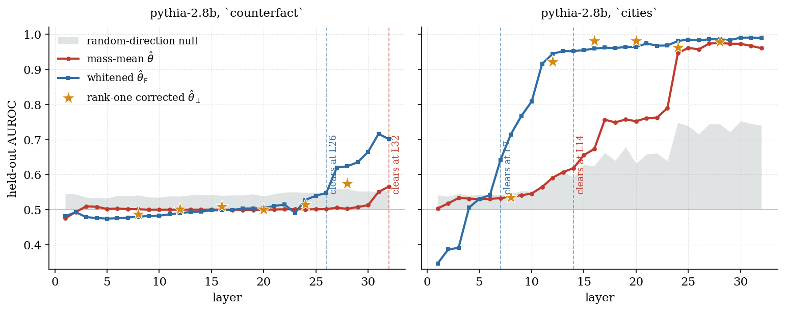
Read against the decoding null, the two datasets separate cleanly, and the correction makes the truth direction recoverable on counterfact. On cities the mass-mean direction leaves the null band at layer \(14\) and stays above every subsequent layer, climbing above \(0.95\) from layer \(25\) and peaking at \(0.975\) at layer \(28\). The whitened direction clears the null earlier, at layer \(7\). On counterfact the mass-mean direction stays inside the null band at every layer but the last, where it reaches \(0.566\) against a null of \(0.556\), while the whitened direction leaves the band at layer \(26\) and climbs to \(0.716\) against \(0.552\) at layer \(31\). The layer-\(32\) value is the maximum of a \(5\%\) test taken over \(33\) layers, so it is a selected extreme rather than a recovery. The rank-one direction \(\hat\theta_\perp\), measured on a six-layer grid in the rogue-dimension sweep, tracks the whitened direction: on counterfact it sits at chance through layer \(24\) and reaches \(0.574\) at layer \(28\), and on cities it is already at \(0.921\) by layer \(12\). Deleting the axis and downweighting it do the same work.

There is a sharper way to explain why the plain probe cannot leave the band on counterfact. When \(\delta\) lies along \(\hat v_1\) and \(\hat v_1\) carries nearly all of \(\hat C\), a random direction \(u\) reads the class gap and the noise through the same coordinate, \(u^{\top}\delta \approx \lVert\delta\rVert u_1\) and \(u^{\top}\hat C u \approx \hat\lambda_1 u_1^{2}\), so

\[d'(u) \;\approx\; \frac{\lVert\delta\rVert\,\lvert u_1\rvert}{\sqrt{\hat\lambda_1}\,\lvert u_1\rvert} \;=\; \frac{\lVert\delta\rVert}{\sqrt{\hat\lambda_1}} \;=\; d'_{\mathrm{mm}} ,\]

and \(u_1\) cancels. For every random direction the projected gap and the projected noise are carried by the same component, so their ratio is the one \(\hat\theta\) itself gives, and the null collapses onto the mass-mean value. The sweep shows it to the third decimal. On counterfact the held-out \(d'_{\mathrm{mm}}\) is \(0.082\), \(0.081\), \(0.081\), \(0.080\) at layers \(8\), \(20\), \(24\), \(28\), and the median of the random-direction null at the same layers is \(0.083\), \(0.081\), \(0.079\), \(0.078\). The plain probe is not merely inside its null. Its \(d'\) is indistinguishable from that of a random direction, and the spread above that median, \(p_{95}\) from \(0.094\) to \(0.139\), is what the two percent of variance off the axis contributes. That is what locked to the axis means operationally, and it is why more data would not lift \(\hat\theta\) clear of the band while the alignment holds: the null and the estimate move together.

\(\hat v_1\) is also well estimated, which is what makes the collapse of \(\hat\theta\) onto it a feature of \(\Sigma\) rather than an accident of the sample. The reason is not the spectral gap by itself. With \(d = 2560\) and \(N = 1198\) the sample covariance is rank-deficient, so no deterministic perturbation bound applies without first controlling \(\lVert\hat C - \Sigma\rVert\), and in this regime a sample eigenvector is in general an attenuated estimate of its population axis. What controls the attenuation is the spike strength relative to the aspect ratio. Writing \(\gamma = d/N = 2.14\) and \(\ell\) for the ratio of \(\hat\lambda_1\) to the bulk scale, the relative bias of \(\hat\lambda_1\) and the squared overlap deficit of \(\hat v_1\) are both of order \(\gamma/\ell\). Taking \(\hat\lambda_2\) as the bulk gives \(\ell = 535\) and \(\gamma/\ell = 4\times10^{-3}\), and taking the mean of the nonzero bulk eigenvalues gives \(\ell = 5.8\times10^{4}\). Either way the spike sits far above the threshold \(1 + \sqrt\gamma = 2.46\), in this ratio convention, below which the leading eigenvector would carry no information about its population axis at all.

Those asymptotics assume rows with bounded fourth moments. The next section shows that this spike is generated by eleven statements out of \(1198\) carrying a single massive coordinate, which violates that assumption, so the spike-strength argument is indicative rather than tight here. That \(\hat v_1\) is a population axis and not a finite-sample artifact rests instead on two direct checks. Identifying the eleven statements coordinate-first, by the size of that one coordinate and without forming the covariance, returns the same eleven at every layer, and a two-point variance formula built from those eleven predicts \(97\)–\(99\%\) of \(\hat\lambda_1\). A direction that can be derived by two disjoint routes is not a finite-sample accident. \(\hat\theta\), by contrast, is a poor estimate of \(\theta\), precisely because the class-gap signal is weak.

The obvious objection is that this is a fact about Pythia. However, the same observables on OLMo-2-1B, a different architecture and training corpus at a third of the parameters, reproduce the pattern. On counterfact the mass-mean direction stays aligned with the leading axis at every depth except the final layer, and the plain probe never clears its null while whitening does, and on cities the alignment falls, the participation ratio climbs, and the plain probe clears the null as it does in Pythia. The numbers are in the appendix Replication on OLMo-2-1B.

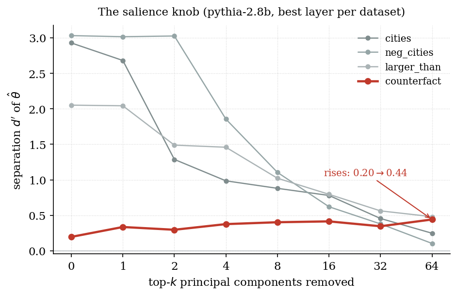
The superposition probe set up in The geometry reads the same object from the other side, and on Pythia it separates the datasets the same way. On cities the separation decays steadily once the leading components go, \(d'_{\mathrm{mm}} = 2.93 \to 0.25\), and larger_than decays likewise. On neg_cities it is untouched until the top two are removed (\(3.03\) at \(k = 2\)) and only then collapses, so its truth direction sits below the most salient axes rather than in them. counterfact_true_false does neither. Its \(d'_{\mathrm{mm}}\) rises, \(0.20 \to 0.44\), so stripping the leading directions makes the truth signal better. companies_true_false exhibits the same effect more strongly, \(d'_{\mathrm{mm}} = 0.17 \to 1.09\) at \(k = 8\) before falling back to \(0.55\) at \(k = 64\). When removing the leading direction improves recovery, that direction is the rogue dimension seen through the superposition probe rather than the spectrum. Datasets without a rogue dimension lose signal when the same components are stripped.

Where the rogue dimension comes from

The definition in the previous section separates the rogue dimension, a property of the within-class covariance, from the massive activation, a property of one coordinate. On counterfact they coincide at layer \(8\), where \(\hat v_1\) carries \(86\%\) of its mass on the massive coordinate, and differ by layer \(28\), where the eigenvector has delocalized across five coordinates. On cities at layer \(28\) the massive activation is present and the rogue dimension is absent. However, the relation is closer than coincidence. On counterfact the leading axis of the covariance is generated by the statements on which the massive activation drops.

A coordinate that is exactly constant across statements contributes nothing to \(\hat C\), however large it is. A coordinate that takes a large value \(a\) on a fraction \(1-p\) of statements and a much smaller value \(b\) on the remaining \(p\) contributes the variance of a two-point distribution,

\[\operatorname{Var}[x_j] \;=\; p(1-p)\,(a-b)^{2},\]

which for small \(p\) and large \(a-b\) can be enormous. At counterfact layer \(8\), four coordinates qualify as massive activations under the magnitude criterion of Sun et al. On each, \(1187\) of the \(1198\) statements sit at a near-constant value and eleven sit far below it. Coordinate \(1793\) reads \(1076.3 \pm 2.7\) on the majority and \(38.4 \pm 2.1\) on the eleven. With \(p = 11/1198\) the formula predicts \(9800\) against a measured coordinate variance of \(9788\). Summed over the four coordinates it gives \(11{,}271\) against \(\hat\lambda_1 = 11{,}413\), and \(\hat v_1\) carries \(98.6\%\) of its mass in their span. At layer \(28\) the same holds with eight such coordinates: \(7249\) against \(\hat\lambda_1 = 7500\), with \(96.6\%\) of \(\hat v_1\) in their span. In this case \(\hat v_1\) carries no truth content. It is, to within a few percent, the indicator of which statements failed to receive the massive activation. The mass-mean estimator’s \(0.994\) alignment with it is an alignment with an eleven-out-of-1198 membership function.

The eleven statements are identifiable coordinate-first, by a rule that never touches the covariance, the class means, or the labels, and it returns the same eleven at every layer. Refitting with them excluded collapses the geometry at layer \(28\), taking \(\hat\lambda_1/\hat\lambda_2\) from \(535\) to \(1.1\) and \(\lvert\cos(\hat\theta,\hat v_1)\rvert\) from \(0.994\) to \(0.063\), and it leaves held-out \(d'_{\mathrm F}\) unchanged at \(0.385\). At that layer whitening leaves nothing further for deletion to recover. Nothing rescues the plain estimator, whose \(d'_{\mathrm{mm}}\) stays inside its null under every removal regime tested. How the eleven are identified, what removing them does to \(d'\) at each layer, and how that comparison depends on the Ledoit–Wolf intensity are given in the appendix Identification and removal of the eleven outlier statements.

The massive coordinates themselves are not dataset-specific. The same coordinates qualify on cities and counterfact alike. What differs is whether any statement drops these coordinates. On cities none do, so the coordinates stay constant, contribute nothing to \(\hat C\), and leave no rogue dimension behind. That is the earlier observation that cities carries the same massive activation without the same pathology, now with a mechanism rather than a coincidence. The incidence is specific to the dataset but the mechanism is general. The per-layer incidence on both models, including pythia-1.4b, is in the appendix Identification and removal of the eleven outlier statements.

While \(\hat\theta\) and \(\hat v_1\) are aligned geometrically, it is unclear whether this is causal. The steering sweep includes a condition that displaces along \(\hat v_1\) itself, the leading eigenvector of the within-class covariance. Because \(\hat v_1\) is fit after both class means are removed, it is defined purely by within-class scatter and carries no information about which statements are true. At layer \(28\) the antisymmetric response to \(\hat v_1\) is \(-0.051\) against \(\hat\theta\)’s \(-0.047\). At layer \(20\) the two agree to within \(10^{-4}\) (\(-0.0390\) against \(-0.0391\)). At every depth measured they track each other to within a few thousandths. They decode alike too, at held-out \(\mathrm{AUROC} = 0.511\) for \(\hat v_1\) against \(0.514\) for \(\hat\theta\) in the six-layer rogue-dimension sweep, both inside the null. The \(0.994\) alignment is a geometric statement. The steering agreement is its behavioral form: a direction fit without any reference to the labels moves the model as much as \(\hat\theta\) does and in the same direction. That establishes that truth content is not what carries the effect. It does not add independent evidence about the size of the effect, since under \(\chi(w) = c\,(w\cdot g)\), derived below, two directions with cosine \(0.994\) must produce nearly equal susceptibilities.

This reframes the anomaly. Steering along \(\hat\theta \approx \hat v_1\) is not steering along truth. It is displacing the activation along the dominant axis of the within-class noise, which perturbs the forward pass in a way that happens to suppress the true completion. A nuisance direction carries no information about the label, so nothing requires its behavioral effect to come out positive. Nothing requires it to be reproducible either, but here it is: the same negative sign appears across ten seeds, at two counterfact layers, and at mid-depth on cities. Whatever produces it is systematic rather than arbitrary, and the label-blindness of \(\hat v_1\) says only that truth is not what produces it.

If that account is right, removing the contribution of \(\hat v_1\) should recover a correctly signed causal effect, by correcting the estimator’s alignment with the rogue dimension rather than by enriching the function class.

What steering measures

Before testing that prediction, it is worth asking what the steering number reports. The susceptibility is a linear functional of the direction pushed. Writing \(g = \big\langle \nabla_x \ell(x)\big\rangle\) for the mean gradient of the behavioral score over the evaluation set, the odd part of the response gives

\[\chi(w) \;=\; \left.\frac{\mathrm{d}A}{\mathrm{d}h}\right|_{h\to 0} \;=\; c\,\big(w \cdot g\big)\]

to leading order, the even terms having been removed by the antisymmetrization. So steering in the small-\(h\) window reports the overlap of \(w\) with the single vector \(g\) along which the model’s true-versus-false margin moves. It does not test whether \(w\) is a truth direction.

Every susceptibility quoted above is therefore a projection of one vector. This is why the \(\hat v_1\) and \(\hat\theta\) measurements agreeing to within \(10^{-4}\) at layer \(20\) is a restatement of their \(0.994\) alignment rather than independent confirmation.

Decomposing in the plane of the next section, \(\hat\theta = \cos\varphi\,\hat v_1 + \sin\varphi\,\hat e_2\), linearity gives

\[\chi(\hat\theta) \;=\; \cos\varphi\;\chi(\hat v_1) \;+\; \sin\varphi\;\chi(\hat e_2),\]

and at \(\cos\varphi = 0.994\) the first term dominates unless \(\chi(\hat e_2)\) is two orders of magnitude larger. One consequence holds before any measurement: a direction that merely disrupts the computation contributes to \(S\), not to \(A\), since \(A\) is odd by construction. A wrong-signed \(A\) therefore requires a signed channel onto the margin, \(\hat v_1 \cdot g < 0\), which the estimator would inherit in proportion to \(\cos\varphi\). Whether that channel exists is a question the gradient answers directly.

This also makes the assumption behind the correction explicit. Projecting out \(\hat v_1\) recovers the sign only if \(g\) has little weight along \(\hat v_1\), i.e. the behaviorally causal direction and the salient axis are close to orthogonal in activation space. When they are not, \(\chi(\hat v_1)\) mixes a truth term with a nuisance term inseparably, so deleting the axis would delete real causal signal along with the artifact.

Measured. One backward pass per example gives \(\nabla_x \ell\), and \(g\) follows by averaging over the same \(250\) contrastive pairs the steering measurements use. Because the gradient is computed per pair, every overlap below carries a bootstrap interval over those pairs rather than resting on the point estimate. I quote \(95\%\) intervals from \(10{,}000\) bootstrap resamples under a fixed seed, and the scale to keep in mind is that a random direction gives \(\lvert\cos\rvert \approx 1/\sqrt{d} = 0.020\) at \(d = 2560\).

At layer \(28\), \(\cos(g,\hat v_1) = -0.011\) with \(95\%\) confidence interval \([-0.038, +0.020]\). The overlap is consistent with zero. That has two consequences. Projecting \(\hat v_1\) out removes essentially none of the behavioral channel, which is what licenses the correction. A channel consistent with zero cannot produce the wrong sign at first order, so \(A(\hat v_1) = -0.051\) at this layer is not a linear effect. It is beyond first order in the displacement.

At layer \(20\) the overlap is resolved: \(\cos(g,\hat v_1) = -0.049\), confidence interval \([-0.061, -0.030]\), and \(\cos(g,\hat\theta)\) is the same through the \(0.994\) alignment. The linear prediction \(c\,(\hat\theta\cdot g) = -0.078\) then lands within about \(20\%\) of the measured \(A(0.5)/0.5 = -0.064\). The through-origin susceptibility hides this, because the response reverses sign with displacement, from \(-0.032\) at \(h = 0.5\) (\(7/10\) seeds negative, \(2.5\) null standard deviations) through zero near \(h = 1\) to \(+0.016\) at \(h = 2\) (\(9/10\) seeds positive), so the slope fit over \(h \le 4\) comes out null. The two layers therefore differ in kind. At layer \(20\) the wrong sign is a first-order effect confined to the linear window. At layer \(28\) the same prediction gives \(-0.002\) against a measured \(-0.039\) at \(h = 0.5\), and the wrong sign persists to \(h = 2\) before its magnitude falls at \(h = 4\).

The overlap with \(g\) also separates the two estimators. On counterfact the whitened direction has a positive overlap at every layer from \(20\) on, \(+0.040\) \([+0.017, +0.056]\) at \(L20\), \(+0.065\) \([+0.034, +0.079]\) at \(L24\) and \(+0.064\) \([+0.028, +0.080]\) at \(L28\), while the plain direction is consistent with zero at \(L24\) and \(L28\). On cities it is the plain direction that has the positive overlap at layer \(28\), \(+0.050\) \([+0.032, +0.062]\), while the whitened direction does not. In both datasets the direction that steers correctly is the direction whose overlap with \(g\) is positive, and the overlap is measured without displacing an activation. The sign and not the magnitude is what carries this: at counterfact layer \(20\) both directions have resolved overlaps, the whitened one positive and the plain one negative.

The rank-one correction gives the sharpest test of this, because \(\hat\theta_\perp\) is exactly \(\hat e_2\), so its susceptibility is predicted by \(\cos(g, \hat e_2)\) alone, measured before anything is steered. On counterfact the prediction has the right sign at all six layers of the rogue-dimension sweep, and where the overlap is resolved the steering is significant and agrees with it. At layer \(8\) the overlap is negative, \(-0.048\) \([-0.062, -0.025]\), the prediction is \(c\,(\hat e_2\cdot g) = -0.12\), and \(\hat\theta_\perp\) steers significantly wrong-signed, \(A(1) = -0.104\) over three seeds (\(p = 0.02\) against a \(100\)-draw null). At layers \(24\) and \(28\) the overlap is positive, \(+0.059\) and \(+0.073\), and \(\hat\theta_\perp\) steers correctly, \(+0.032\) and \(+0.043\) against a predicted \(+0.054\) at both. At layers \(12\) through \(20\) the overlap’s interval spans zero and the steering stays inside its null. Removing \(\hat v_1\) corrects the sign only where what remains of the class gap overlaps \(g\) positively.

cities also reproduces the mid-depth dip from the other side. Its plain overlap turns significantly negative at layer \(20\), \(-0.035\) \([-0.041, -0.027]\), which is the same window where the steering sweep finds \(\chi = -0.0062\), an independent confirmation of an anomaly that the steering measurement alone left uncertain.

There is a geometric reading of the two directions that makes the inversion of Marks & Tegmark’s assignment in The geometry less paradoxical than it first appears. A readout is a covector and a steering direction is a vector. To first order a displacement couples to one covector, the score gradient \(g\), so a direction steers correctly when it overlaps \(g\). Marks & Tegmark’s assignment is to steer along \(\delta\) and read with \(\Sigma^{-1}\delta\). This is right whenever \(\delta\) overlaps \(g\), which is the case on cities. On counterfact, \(\hat\delta\) lies along a nuisance axis with no overlap with \(g\). \(\Sigma^{-1}\) removes that axis and restores the overlap. This does not show that the model’s own readout is closer to \(\Sigma^{-1}\delta\) than to \(\delta\) in general. On cities the plain direction carries the overlap but the whitened one does not.

Two cautions on reading these magnitudes, the curvature at the large-\(h\) end and how much of \(g\) the plane captures, are given in the methods appendix.

The correction is a rotation in a plane

Two corrections to the estimator, whitening and projecting out \(\hat v_1\), make the same prediction, and neither adds capacity. Whitening replaces \(\hat\theta \propto \hat\delta\) with the Fisher direction \(\hat\theta_{\mathrm F} \propto \hat\Sigma^{-1}\hat\delta\), which downweights the mean-shift component along high-variance axes, \(\hat v_1\) chief among them. The blunter control simply projects \(\hat v_1\) out, \(\hat\theta_\perp \propto (I - \hat v_1 \hat v_1^{\top})\hat\delta\), removing only the rogue dimension.

The two look like corrections of different rank, since the projection is exactly rank one while \(\hat\Sigma^{-1}\) is not. However, in this regime they act inside the same plane. Letting \(P = \mathrm{span}\{\hat v_1, \hat e_2\}\) with \(\hat e_2 = \hat\delta_\perp / \lVert \hat\delta_\perp \rVert\) defined as the unit vector along the part of the class gap orthogonal to the rogue axis, \(\delta_1\) and \(\delta_\perp\) can be written as \(\delta_1 = \hat v_1^{\top}\hat\delta\) and \(\delta_\perp = \lVert\hat\delta_\perp\rVert\) respectively. \(\hat\Sigma\) can be restricted to \(P\) as \(\mathrm{diag}(\lambda_1, \bar\lambda)\). For a unit direction in the plane \(u(\varphi) = \cos\varphi\,\hat v_1 + \sin\varphi\,\hat e_2\), the separation it achieves is a Rayleigh quotient in the single angle \(\varphi\):

\[d'^{2}(\varphi) \;=\; \frac{(\delta_1\cos\varphi + \delta_\perp\sin\varphi)^{2}} {\lambda_1\cos^{2}\varphi + \bar\lambda\sin^{2}\varphi}.\]

The mass-mean estimator sits at \(\tan\varphi_{\mathrm{mm}} = \delta_\perp/\delta_1\) and the Fisher direction has plane components \((\delta_1/\lambda_1,\ \delta_\perp/\bar\lambda)\), so the two are related by a single lever arm \(\kappa \equiv \lambda_1/\bar\lambda\):

\[\tan\varphi_{\mathrm F} \;=\; \kappa \tan\varphi_{\mathrm{mm}} .\]

This shows that whitening is simply a rotation within \(P\). The measured \(\lvert\cos(\hat\theta,\hat v_1)\rvert = 0.994\) puts \(\varphi_{\mathrm{mm}} = 6.3^{\circ}\). With \(\kappa = \hat\lambda_1/\hat\lambda_2 = 535\) this gives \(\varphi_{\mathrm F} = 89.0^{\circ}\). These are full-sample values of \(\hat C\). The whitening actually applied uses the shrunk \(\hat\Sigma\) of the training half, where \(\kappa = 463\) and \(\varphi_{\mathrm{mm}} = 6.8^{\circ}\), and it returns the same \(89.0^{\circ}\) and the same predicted gain below. The whitened direction is orthogonal to \(\hat v_1\) to within a degree, which is why \(\hat\theta_{\mathrm F}\) and \(\hat\theta_\perp\) produce the same sign flip: in this regime they are the same vector, and the full-rank correction reduces to the rank-one one.

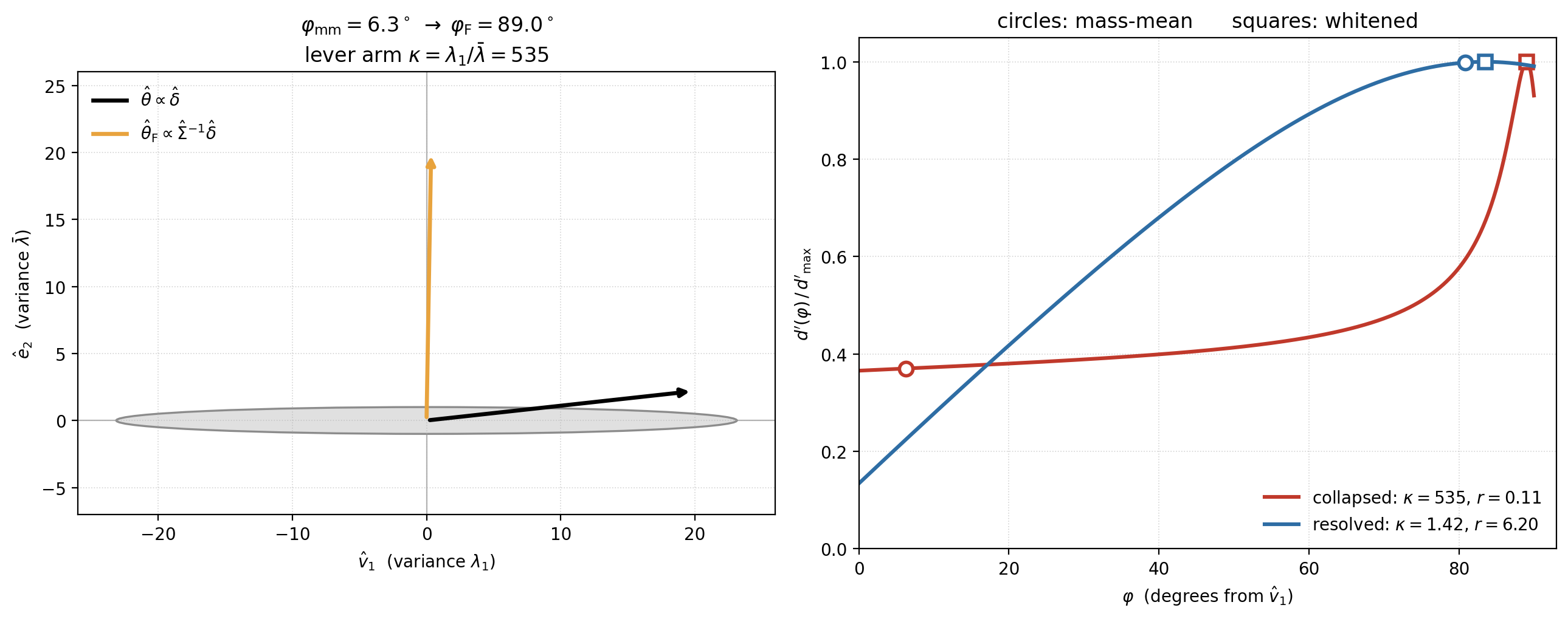
The quotient also predicts the size of the gain. Writing \(r = \tan\varphi_{\mathrm{mm}}\),

\[\frac{d'^{2}_{\mathrm F}}{d'^{2}_{\mathrm{mm}}} \;=\; \frac{(\kappa^{-1} + r^{2})(\kappa + r^{2})}{(1+r^{2})^{2}} \;\approx\; \frac{1 + \kappa r^{2}}{(1+r^{2})^{2}},\]

which at \(\kappa = 535\) gives \(2.7\times\). Measured on counterfact at layer \(28\), \(d'_{\mathrm{mm}} = 0.080 \to d'_{\mathrm F} = 0.384\), a factor of \(4.8\). The formula predicts the right order and underestimates the measured gain. Inverting it for an effective \(\kappa\) is worked through in the methods appendix, under The \(\kappa_{\mathrm{eff}}\) inversion.

Two conditions make the reduction valid, and together they are the criterion for this failure mode. The spectrum must have one dominant eigenmode, \(\mathrm{PR} \approx 1\) with \(\lambda_1/\lambda_2 \gg 1\), or there is no plane to reduce to. Additionally, \(\varphi_{\mathrm{mm}}\) must be small, or the estimator is not at the foot of the cliff and there is nothing to correct. Both are read off the activations and the fitted direction, and together they diagnose that the estimator has collapsed onto \(\hat v_1\). They do not by themselves say which way either direction will steer. That is set by the overlaps with the score gradient, \(\hat v_1\cdot g\) for the mass-mean direction and \(\hat e_2\cdot g\) for the correction, which are also measured without displacing an activation. At counterfact layers \(8\) through \(16\) the spectrum meets the criterion more strongly than at layer \(28\), yet the corrections do not restore the sign there, because \(\hat e_2\cdot g\) is negative or unresolved. The diagnosis from the spectrum and the sign from the gradient are both available before any steering is run. The diagnosis has been tested on one dataset (counterfact) that satisfies the criterion, and one (cities) that does not, and held in both. Two further main-tier sets, companies_true_false and common_claim_true_false, satisfy the criterion at layers \(24\) and \(28\) but cannot be tested causally with this harness. Their statements have no relation structure from which to build a pair of completions, so the behavioral score of The scale of an intervention cannot be formed. The alternative would be to score the model’s own judgment of whether a statement is true, but unsteered that judgment separates true from false at AUROC \(0.57\) on common_claim, against \(0.78\) on cities, so there is almost no behavior there for a displacement to move. So they meet the criterion, but the prediction it makes for them cannot be checked. cities at layer \(28\) violates both conditions (\(\mathrm{PR} = 29.7\), \(\lvert\cos\rvert = 0.159\)). There the formula predicts a gain of \(1.00\times\) at \(\kappa = 1.42\) and \(r = 6.2\), since both directions already sit on the broad top of the quotient, and the measured \(1.22\times\) is a small gain from the rest of the spectrum, outside the plane. The formula stops applying where the regime ends, and the regime control below draws the same boundary.

Both corrections flip the sign. Steering along the whitened direction at layer \(28\) gives

\[A(1) > 0 \;\text{ in } 10/10 \text{ seeds}, \qquad \operatorname{med}_{\text{seeds}} A(1) = +0.025 = 2.1\,\sigma_{\text{null}}, \qquad p = 0.010,\]

with \(8/10\) seeds individually clearing the null at \(5\%\). Layer \(24\) gives the same picture: \(10/10\) positive, \(7/10\) clearing, \(p = 0.020\). Here \(\chi\) coincides with \(A(1)\) at \(+0.025\), because the whitened response is linear in \(h\) over the whole sweep, \(0.013\), \(0.025\), \(0.050\), \(0.099\) at \(h = 0.5, 1, 2, 4\), where the plain direction’s response fell off at \(h = 4\). The corrected effect is smaller than the wrong-signed one it replaces, two null standard deviations against five, but it is monotone where that one was not. The rank-one correction \(\hat\theta_\perp\), measured independently in the rogue-dimension sweep, agrees. At layer \(28\) its three seeds give \(A(1) = +0.045\), \(+0.036\) and \(+0.048\), each at \(p \le 0.0025\) against the same \(400\)-draw null, so on its own it carries \(A\) from significantly negative to significantly positive, and it raises held-out decoding AUROC at layer \(28\) from \(0.51\), the mass-mean value inside the null, to \(0.57\). Layer \(20\) is the crossover. Whitened steering there is correctly signed in \(9/10\) seeds but does not clear the null, \(p = 0.12\), which corresponds to a transition region rather than a clean effect.

The regime control

Marks & Tegmark steer along the feature direction and report that difference-in-means directions are the most causally implicated of the probes they compare. At the deep counterfact layers that ordering reverses. The mass-mean direction, which their framework nominates as the feature, steers the model away from the true completion, and the whitened direction, which it demotes to a decision boundary, steers the model toward it. The rogue-dimension diagnosis explains why. There \(\hat\theta\) has collapsed onto \(\hat v_1\) and is not tracking a feature at all, so the \(\Sigma^{-1}\) meant to sharpen a readout is instead doing the work of recovering the direction.

The inversion is a property of a regime, not a refutation of Marks & Tegmark, which is demonstrated by cities as a the control. There the two directions behave as mass-mean probing intends. At pythia-2.8b layer \(28\), the same model and depth at which counterfact inverts, the plain direction steers correctly in \(10/10\) seeds (\(\chi = +0.030\)) while the whitened direction is weak and inconsistent (\(\chi = -0.003\), \(4/10\)). On pythia-1.4b the contrast is starker still, with \(\chi = +0.46\) plain against \(-0.013\) whitened at layer \(12\). Read across the whole depth sweep, the two datasets mirror each other. On cities, plain steering clears its null at three layers, \(12\) and \(28\) clearly and \(24\) weakly (\(\chi = +0.009\), \(10/10\) seeds positive, \(p = 0.020\)), and is correctly signed at all three. On counterfact, plain steering clears its null at two layers, \(24\) and \(28\), and is wrong-signed at both. At every other layer of either dataset it sits inside the null. At layer \(28\) the two datasets share the model, the depth and the estimator, and their significant effects point in opposite directions. When no single eigenmode dominates the within-class covariance, the mean difference is the causal feature and the inverse covariance only adds estimation noise, which is what Marks & Tegmark report, on datasets of exactly this kind. The inversion is confined to the regime where \(\hat\delta\) has collapsed, and the rogue dimension decides which regime a dataset is in.

Two points in the cities panel deserve naming, since they are visible and read at first glance like counterexamples. At layers \(16\) and \(20\) the plain direction becomes mildly negative with \(\chi = -0.0031\) and \(-0.0062\). Both estimates are consistent across seeds (\(9/10\) and \(8/10\) negative), so the sign is not noise. However, both sit an order of magnitude below the \(+0.0296\) the same direction produces at layer \(28\), and neither clears the steering null. The regime claim is that the significant effects on cities are correctly signed, not that every layer’s point estimate is positive.

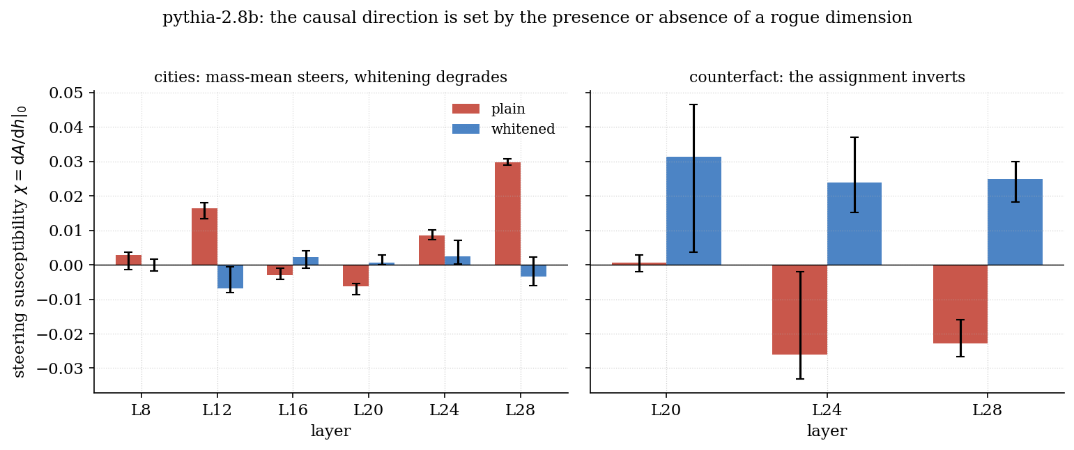
Discussion

The results above establish that, when the within-class spectrum meets a specific criterion, the mass-mean estimator returns a nuisance direction rather than a truth direction, and that a correction inside the linear class restores the sign of the steering effect along the corrected direction. Two things should be noted before comparing to other reports. The first is the magnitude of the corrected effect, and the second is what its success does and does not imply about the function class.

The corrected effect is modest. At one class gap the plain direction’s median response is \(-0.062\), five null standard deviations, and the whitened direction’s is \(+0.025\), two. The correction flips the sign of the effect but returns less than half its size. The decoding gain is likewise real but small in absolute terms. Whitening carries held-out AUROC at layer \(28\) from \(0.502\), inside the null, to \(0.624\) against a null of \(0.560\), and the whitened direction stays clear of its null from layer \(26\) to the end of the network, peaking at \(0.716\) against \(0.552\) at layer \(31\). Set beside cities, where the same direction reads \(0.99\), this is a weak readout. The overall claim is a corrected sign and a confirmed mechanism, not a recovered truth direction of practical use.

A wrong-signed steering effect invites a natural reading that the linear function class is too weak: the direction one can fit is not expressive enough to move behavior, and a richer, perhaps nonlinear, intervention is required. The rogue-dimension account makes a different claim about this particular failure. The class is adequate, but the mass-mean estimator points at \(\hat v_1\), a massive-activation direction, instead of at truth. The two readings make different predictions, and the data separate them. A rank-one correction within the same linear class, with no richer classifier and no nonlinear probe, converts a wrong-signed effect that clears its null into a correctly signed one that clears its null. For the counterfact failure at layers \(24\) and \(28\) the function class was never the bottleneck. The estimator’s alignment with a massive-activation direction was.

Relation to other reports

Four recent reports also examine why a fitted direction fails to steer, and the rogue-dimension account can be compared against each. Braun et al. and Ying et al. locate the failure in the direction. For Braun et al. steering is unreliable when the per-example activation differences do not point the same way, so that their mean is not representative of any of them. For Ying et al. steering is wrong-signed when the direction is fitted across many kinds of truth and mixes truth with sycophancy. Torop et al. find a direction that discriminates well and steers backwards. Liu finds a direction that decodes but does not steer at all. This post shares a predictor with the first two and differs on the diagnosis, and against the last two it supplies the remaining case, a direction that neither decodes nor steers correctly.

Braun et al. (2025) study contrastive activation addition across thirty-six behaviors and find two predictors of whether steering works: the mean pairwise cosine similarity among the per-example activation differences, which measures whether those differences share a direction, and the separability of positive from negative activations along the difference-of-means line. Their separability index is the discriminability \(d'\) of the projection onto that line, which is the \(d'_{\mathrm{mm}}\) of this post. While these two reports share a predictor, they differ in what they find at low \(d'_{\mathrm{mm}}\). Every dataset in Braun et al.’s study steers with a net positive effect, with low separability showing up as per-example scatter around that mean. In those cases they conclude that the behavior is not represented by a coherent linear direction. counterfact at layers \(24\) and \(28\), with \(d'_{\mathrm{mm}} = 0.08\), sits at the unsteerable end of their scale but steers with a negative mean that clears its null. This implies that the behavior is linearly represented, since the whitened direction steers it correctly at the same layer. What has failed is the estimator. The superposition result above is the decoding-side form of the same failure, a high-variance direction interfering with the target signal, whose removal improves recovery. The shallow counterfact layers, \(L \le 16\), are closer to the regime Braun et al. describe, but not the same one. Whitening leaves the effect inside the null there, and projecting out \(\hat v_1\) does not restore the sign: at layer \(8\) it steers significantly wrong-signed. That is not an absence of linear signal. It is the sign of \(\hat e_2\cdot g\), which at that depth is negative, as What steering measures shows. The per-sample form of the anomaly is documented by Tan et al. (2024), who find that for several concepts close to half the inputs steer in the direction opposite to the one intended. The counterfact effect at layers \(24\) and \(28\) is that variance surfacing as a wrong-signed dataset-level mean that clears its null, with a proposed mechanism.

Ying et al. (2026) compare two kinds of truth direction: domain-specific ones, each fitted within a single truth type, and a domain-general one recovered by concept erasure across many truth types. Steering along a domain-specific direction improves truthfulness on held-out factual questions. Steering along the domain-general one consistently degrades it. Their account is one of mixture: a direction trained to span many domains conflates factual variance with sycophancy-related variance, so intervening along it moves several things at once. That mechanism is not available here, since the estimator is fitted on the counterfact domain alone and there is no second domain to mix in. Within that one domain the class-mean difference is small compared with the spread along the leading within-class eigenmode, and the estimator returns that eigenmode rather than the truth direction. The two results therefore agree that a direction fitted to truth can steer against it but disagree on the mechanism and on the remedy. Theirs is to fit within a single truth type. The remedy here is to keep the fitted direction and project out one eigendirection before reading it.

Torop, Masoomi & Dy (2026) find inverted steering vectors in the attention-head outputs of Gemma 3 12B, Qwen 2.5 14B and Olmo 3 7B: mean-difference directions that discriminate the concept well, \(\mathrm{AUC} \ge 0.85\) by their candidate cutoff, and whose positive steering consistently suppresses it across inputs. They separate this from Tan’s per-input anti-steerable examples and from the low-discriminability failures Braun et al. describe. Their inversion comes with a direction that decodes well while the counterfact inversion comes with a nuisance direction that fails to decode, since \(\hat\theta\) sits inside its decoding null. The mechanism found here, alignment with a label-blind variance axis, is unavailable when the direction is discriminative. The two are the same failure of sign at opposite ends of decodability, and the diagnostics differ accordingly. They diagnose it through a downstream inner-product response, while this post reads the spectrum of the within-class covariance. Whether the rogue-dimension criterion says anything about their cases is open.

Liu (2026) finds an overthinking failure in medical QA that is linearly decodable at \(71.6\%\) balanced accuracy. Liu subsequently finds that five families of fixed residual-stream linear steering, across twenty-nine configurations, all move the behavior by nothing measurable. This is the decode-without-cause shape arrived at from the other side, and Liu attributes it to representational entanglement. Two things separate it from the case here. The effect described by Liu is null rather than wrong-signed, so there is no sign to restore. The entanglement is inferred from the failure, whereas the nuisance direction responsible here is named in advance from the within-class spectrum and then removed. A null steering result cannot distinguish an entangled direction from one that is absent, while a significantly wrong-signed result with an identified direction can.

Summary

A mass-mean truth direction can either be a truth direction or the estimator’s projection onto the most salient axis of the activations. On a benchmark the two are told apart only by a signal-to-noise reading. Three results follow. In-sample separation is inflated by dimensional slack that scales as \(N^{-1/2}\) with a prefactor set by the effective dimension of the noise, meaning that for the datasets in this literature the null and not the raw score is the bar. When the class gap is weak the mass-mean estimator collapses onto the leading within-class eigenvector. On counterfact that direction fails to decode and steers with a significant wrong sign, five null standard deviations deep at one class gap. The failure is in the estimator: the same activations used to obtain the mass-mean direction contain a direction that steers correctly, and it can be reached without leaving the linear class, either by the Fisher direction or by projecting out the leading eigenvector.

The results have limits. The criterion that diagnoses this failure, a within-class spectrum with one dominant eigenmode and the mass-mean direction aligned to it, has one confirmed positive and one confirmed negative. It identifies the collapse but not the sign of a correction, which is set by the overlap of the corrected direction with the score gradient. The steering measurements are on Pythia alone, since OLMo replicates the geometry and the decoding but was not steered. The wrong sign at layer \(28\) is beyond first order in the displacement and its mechanism is not settled here. The corrected effect is modest. The whitened direction’s response at one class gap is two null standard deviations, where the wrong-signed response of the mass-mean direction was five, so the correction restores a sign rather than supplying a large causal lever. On one of four datasets the shuffled-label amplitude departs from the parameter-free prediction by \(36\)–\(60\%\) for reasons that were localized but not explained.

This post has treated steering as a diagnostic. The steering results themselves are analyzed in a second, forthcoming post, Steering Vectors and the Limits of Linear Response. There the object of interest is the vector \(g\) itself. Starting from the identity \(\chi(w) = c\,(w\cdot g)\), I ask how much of \(g\) lies along the high-variance directions of the within-class covariance, what bound it puts on any linear steering direction, how much of that bound the best direction actually reaches, and how much of \(g\) published steering vectors capture.

Appendix: AUROC and its relation to \(d'\)

The main text defines \(\mathrm{AUROC}(u) = \Pr[z_1 > z_0]\) as the probability that a random true statement outscores a random false one. This is the quantity the random-direction null resamples. The name refers to a different construction, the area under the receiver-operating-characteristic curve. This appendix builds that curve, shows its area equals the scoring probability, and records the Gaussian special case behind \(\mathrm{AUROC} = \Phi(d'/\sqrt{2})\). The same Gaussian link, together with a closed form for the Mahalanobis cosine as a function of \(d'\), is derived by Ying, Hase & Kriegeskorte (2026), whose signal-to-noise ratio is \(d'(u)\) under the pooled within-class covariance.

The receiver operating characteristic is an inheritance from WWII radar and quantified how well a receiver’s operator could separate signal (an aircraft echo) from noise as the detection threshold was varied. The same curve was adopted wholesale by signal detection theory and then by psychophysics and statistics, which is why a truth-probe analysis and a 1940s radar set share an acronym.

Fixing a direction \(u\) and reading the scalar \(z = u^{\top}x\), a classifier is obtained by thresholding, \(\hat y = \mathbb{1}[z > t]\), and sweeping the threshold \(t\) from \(+\infty\) to \(-\infty\) traces out two functions of \(t\):

\[\mathrm{TPR}(t) = \Pr[z > t \mid y=1], \qquad \mathrm{FPR}(t) = \Pr[z > t \mid y=0].\]

Plotting the point \((\mathrm{FPR}(t), \mathrm{TPR}(t))\) as \(t\) sweeps traces out a curve from \((0,0)\) to \((1,1)\). A direction that separates the classes lifts the curve above the diagonal: at every false-positive rate the true-positive rate is higher, so the curve passes near the top-left corner. A useless direction gives the diagonal \(\mathrm{TPR} = \mathrm{FPR}\) itself. The AUROC is the area under this curve. It is \(1\) for perfect separation, \(\tfrac{1}{2}\) for the diagonal, and \(\mathrm{AUROC}(-u) = 1 - \mathrm{AUROC}(u)\) since changing the sign of \(u\) swaps the conditional distributions.

The geometric area and the probabilistic \(\Pr[z_1 > z_0]\) are the same number, which the main text leans on. Writing the class-conditional densities as \(p_1(z) = p(z\mid y=1)\) and \(p_0(z) = p(z\mid y=0)\), with CDFs \(F_1, F_0\), one can parametrize the curve by \(t\): the height is \(\mathrm{TPR}(t) = 1 - F_1(t)\) and the horizontal coordinate is \(\mathrm{FPR}(t) = 1 - F_0(t)\), so \(\mathrm{d}(\mathrm{FPR}) = -p_0(t)\,\mathrm{d}t\). The area, integrated as \(\mathrm{FPR}\) runs \(0 \to 1\) (i.e. \(t\) runs \(+\infty \to -\infty\)), is

\[\mathrm{AUROC} = \int_0^1 \mathrm{TPR}\;\mathrm{d}(\mathrm{FPR}) = \int_{-\infty}^{\infty} \big(1 - F_1(t)\big)\, p_0(t)\,\mathrm{d}t .\]

Reading \(1 - F_1(t) = \Pr[z_1 > t]\) for an independent draw \(z_1 \sim p_1\), the integral averages this over \(t \sim p_0\):

\[\mathrm{AUROC} = \mathbb{E}_{z_0 \sim p_0}\!\big[\Pr[z_1 > z_0]\big] = \Pr[z_1 > z_0],\]

the probability that a random positive outscores a random negative — the Wilcoxon– Mann–Whitney identity. Ties contribute a boundary term of measure zero for continuous \(z\), and half a count apiece if one insists on discrete scores. This is also why AUROC is calibration-free: it depends only on the ordering of scores, not their scale or location, so any strictly monotone reparametrization of \(z\) leaves it unchanged — in particular it needs no choice of threshold, unlike accuracy.

When the class-conditionals of \(z\) are Gaussian and the classes balanced, \(z_y \sim \mathcal{N}(u^{\top}\mu_y,\; u^{\top}\Sigma u)\), the difference \(z_1 - z_0 \sim \mathcal{N}(u^{\top}\delta,\; 2\,u^{\top}\Sigma u)\), so \(\Pr[z_1 > z_0] = \Phi\big(u^{\top}\delta/\sqrt{2\,u^{\top}\Sigma u}\big) = \Phi(d'/\sqrt2)\), recovering the identity quoted in the definitions. Away from that case the map between \(d'\) and AUROC is only approximate, which is why the main text reports both rather than deriving one from the other.

Appendix: results on the full twelve-dataset benchmark

The main text carries cities and counterfact through the steering and rogue-dimension analysis and the nine main-tier sets through the transfer matrix. The sweep covers all twelve. At pythia-2.8b, each at its own selected layer:

dataset	\(L\)	plain AUROC	\(d'_{\mathrm{mm}}\)	whitened AUROC	null \(p_{95}\)
neg_cities	25	0.978	3.03	0.981	0.683
sp_en_trans	27	0.980	2.68	0.974	0.673
neg_sp_en_trans	28	0.974	2.83	0.994	0.677
cities	29	0.973	2.93	0.983	0.721
smaller_than	31	0.974	2.79	1.000	0.786
larger_than	28	0.929	2.05	1.000	0.735
cities_cities_disj	29	0.836	1.42	0.836	0.586
cities_cities_conj	26	0.810	1.30	0.930	0.597
common_claim_true_false	31	0.757	0.64	0.722	0.611
companies_true_false	31	0.699	0.17	0.855	0.585
counterfact_true_false	32	0.566	0.20	0.701	0.556
likely	12	0.890	1.75	0.929	0.593

The two translation sets sit at \(N = 354\) rather than \(1198\) and clear their null by as wide a margin as the single-frame sets. The ordering is informative. Every templated set with a single frame clears its null comfortably. The two free-form sets are the bottom of the table: common_claim_true_false at \(d'_{\mathrm{mm}} = 0.64\) and counterfact_true_false at \(0.20\). companies_true_false is the interesting entry — a plain \(d'_{\mathrm{mm}}\) of \(0.17\), at the floor with counterfact, but a whitened AUROC of \(0.855\), the largest gap between the two estimators anywhere in the table. Together with its rising superposition curve, that makes it a second instance of the rogue-dimension pattern, decoded rather than steered: the dataset ships only statements and labels, with no contrastive completions from which to build a behavioral score, so it carries no causal measurement. The spectrum confirms it. At layers \(24\) and \(28\), companies_true_false has \(\mathrm{PR} = 1.01\) and \(1.02\), \(\hat\lambda_1/\hat\lambda_2\) near \(2000\) and \(1250\), and \(\lvert\cos(\hat\theta,\hat v_1)\rvert = 0.98\) and \(0.93\), with \(d'_{\mathrm{mm}}\) of \(0.02\) and \(0.03\). That is counterfact’s signature at the same depths. By layer \(31\), where selection lands, it has escaped: \(\mathrm{PR} = 3.2\), the alignment down to \(0.18\), \(d'_{\mathrm{mm}}\) up to \(0.51\). common_claim_true_false is a third instance, locked at layers \(24\) and \(28\) (\(\mathrm{PR} = 1.02\) and \(1.05\), alignment \(0.95\) and \(0.83\)) and escaping by layer \(31\) (\(\mathrm{PR} = 12.1\), alignment \(0.21\)). cities_cities_conj, by contrast, never locks (\(\mathrm{PR}\) from \(20\) to \(42\) across the same layers, alignment below \(0.11\)). So within Pythia the rogue dimension is a property of at least three of the nine main-tier sets at mid-depth, and what separates the other two from counterfact is that their class gap grows enough to leave the axis before the network ends, where counterfact’s does not.

One caution about the companies_true_false row is that \(d'\) of \(0.17\) maps to \(\mathrm{AUROC} \approx 0.55\) under the Gaussian identity, not the \(0.699\) measured — the largest departure in the table, and a sign that the projected class-conditionals on this dataset are far from that idealization.

Appendix: identification and removal of the eleven outlier statements

The eleven statements are identifiable without reference to \(\hat v_1\). Selecting outliers by their projection onto \(\hat v_1\) and then recomputing \(\hat v_1\) without them would be circular since removing the top of a distribution shortens it. Instead, the set is defined coordinate-first, without referring to the covariance, the class means, or the labels. A coordinate is massive if \(\lvert\operatorname{med}_i x_{ij}\rvert\) exceeds both an absolute threshold and a large multiple of the median activation, and a statement is flagged if it deviates from the modal value on any massive coordinate. This criterion returns exactly the eleven statements of the projection-based set, at every layer measured. Layer-invariance makes it a property of the input rather than of any particular representation.

Refitting on a training half with the eleven excluded and scoring on the full held-out half leaves the mass-mean direction where it was and moves the whitened one substantially at early and middle depth:

layer	\(d'_{\mathrm F}\), all	\(d'_{\mathrm F}\), eleven removed	null \(p_{95}\)
\(8\)	\(0.010\)	\(0.129\)	\(0.094\)
\(12\)	\(0.015\)	\(0.162\)	\(0.092\)
\(16\)	\(0.031\)	\(0.163\)	\(0.095\)
\(20\)	\(0.005\)	\(0.385\)	\(0.097\)
\(24\)	\(0.063\)	\(0.136\)	\(0.132\)
\(28\)	\(0.384\)	\(0.385\)	\(0.128\)

\(d'_{\mathrm{mm}}\) stays inside its null under every regime, so nothing here rescues the plain estimator. The layer-\(28\) row is the informative one. Removing the eleven moves the geometry enormously there — \(\hat\lambda_1/\hat\lambda_2\) falls from \(535\) to \(1.1\) and \(\lvert\cos(\hat\theta,\hat v_1)\rvert\) from \(0.994\) to \(0.063\) while \(d'_{\mathrm F}\) does not move at all. At that depth whitening has the same effect on \(d'_{\mathrm F}\) as deleting the contaminated statements, but from layers \(8\) through \(20\) whitening alone leaves \(d'_{\mathrm F}\) inside its null, while explicit removal lifts it above the null by factors of \(1.4\)–\(4\). Layer \(24\) sits between the two regimes.

The difference between the two regimes is controlled by the shrinkage intensity. Sweeping \(\rho\) on the uncleaned data reproduces most of the effect of deleting the eleven: at layer \(16\), \(d'_{\mathrm F}\) runs from \(0.031\) at the Ledoit–Wolf \(\rho = 0.137\) to \(0.530\) at \(\rho = 10^{-4}\). What limits \(\hat\Sigma^{-1}\) at these depths is therefore not the contamination itself but the regularization. At the Ledoit–Wolf intensity the estimate is pulled far enough toward the isotropic target that the inverse barely downweights the leading directions. The methods appendix states this as a general point about \(\rho\) — in the note that the whitened numbers are a lower bound — rather than as one about these eleven statements.

The massive coordinates are not dataset-specific. At pythia-2.8b the same four coordinates qualify at layers \(8\)–\(16\), the same seven at layer \(20\) and the same eight at layers \(24\)–\(28\), on cities and counterfact alike. What differs is whether any statement drops them: on cities, none do, at any layer in either model. The coordinates therefore stay constant, contribute nothing to \(\hat C\), and leave no rogue dimension behind. On pythia-1.4b no coordinate qualifies through layer \(15\). One does at layers \(18\) and \(21\), where three counterfact statements drop it, none of them among the eleven and two of the three shared between the layers, and cities again has none. There \(\hat\lambda_1/\hat\lambda_2\) moves only from \(1.5\) to \(1.4\). So the incidence is specific and the mechanism is general. Wherever a near-constant massive activation is dropped by a small minority of inputs, the within-class covariance acquires a rogue dimension whose scale is set by \(p(1-p)(a-b)^2\), and where it is dropped by none, it acquires nothing. I do not know what distinguishes the eleven. They span both labels, all end in a period, and their token lengths sit inside the bulk of the distribution.

Appendix: replication on OLMo-2-1B

To check that the rogue dimension is not a fact about Pythia, I ran the observables of The rogue dimension on OLMo-2-1B, which has a different architecture, a different training corpus and a third of the parameters. counterfact stays locked to the leading axis at every depth except the final layer, \(\lvert\cos(\hat\theta,\hat v_1)\rvert\) between \(0.64\) and \(0.94\) from layer \(2\) to layer \(15\) (it falls to \(0.04\) at layer \(16\)), with \(d'_{\mathrm{mm}} \approx 0.1\). Its plain probe never clears its own null (held-out \(\mathrm{AUROC} = 0.529\) at its best layer, against a null 95th percentile of \(0.547\)), while whitening lifts it to \(0.647\). cities clears the null, as it does in Pythia: the alignment falls to \(\lvert\cos\rvert \approx 0.3\), the participation ratio climbs \(1.4 \to 17.7\), and the plain probe reaches \(0.903\). The superposition probe agrees from the other side. Stripping the leading components raises \(d'_{\mathrm{mm}}\) on counterfact (\(0.07 \to 0.31\)) and destroys it on cities (\(1.85 \to 0.54\)).

Appendix: methods in detail

Everything below describes what the code does, not what the method ideally would do. Where the two differ the difference is stated. Script names refer to the public repository, jasteinberg/rl-alignment-repo, which holds the scripts below, the shared library they import, and the committed artifacts each number is read from.

Models and activations. Pythia 70m, 410m, 1.4b and 2.8b, and OLMo-2-1B for the cross-family check, run in float16 on Apple silicon (MPS) through HuggingFace transformers. The activation \(x\) for a statement is the residual stream at the final token, taken from every layer in one pass via output_hidden_states. Layer \(L\) means the output of block \(L\), and layer \(0\) is the embedding.

Environment. Python 3.11.15, torch 2.10.0 with the MPS backend, transformers 4.57.6, numpy 1.26.4, scipy 1.17.1, scikit-learn 1.8.0, on macOS 26.5.2 (arm64). The backend matters more than usual: MPS kernels have changed numerical behavior between torch releases, so exact reproduction of third-decimal figures should pin these versions.

Data. The nine main-tier sets are capped at \(1199\) and class-balanced, giving \(N = 1198\), the two translation sets sit at \(N = 354\) (their natural size), and likely is carried as a distractor. Caps are applied before splitting, so every dataset in a comparison contributes the same \(N\).

Transfer. A direction is fit on the source’s training half at the source’s selected layer and scored on the target’s held-out half at the target’s selected layer, so the two ends of a transfer sit at different depths whenever the selected layers differ. The diagonal is scored the same way and is held-out.

Split and estimators. One class-stratified \(50/50\) split at seed \(0\) (split_indices), fit on the training half and scored on the held-out half unless a quantity is explicitly marked in-sample. The three directions are

\[\hat\theta \propto \hat\delta, \qquad \hat\theta_{\mathrm F} \propto \hat\Sigma^{-1}\hat\delta, \qquad \hat\theta_\perp \propto (I - \hat v_1\hat v_1^{\top})\hat\delta ,\]

each normalized, and each sign-oriented so that its training-half AUROC is at least \(\tfrac12\). This is necessary because \(d'\) is sign-blind and AUROC is not. \(\hat\Sigma\) is the within-class covariance with each class centered on its own mean, under Ledoit–Wolf shrinkage toward \((\operatorname{tr}\hat C/d)\,I\). The raw \(\hat C\) is singular whenever \(N_{\text{train}} < d\), which is most of this study.

Nulls. The decoding null draws \(200\) random unit directions per layer (Gaussian, then normalized) and scores them on the same held-out points as the fitted direction, so the comparison is not confounded by the split. (The null-distribution figure above draws its own \(400\) in-sample directions on the full set, as an illustration of the distribution’s shape. The \(200\)-draw held-out null is the one every quoted number is scored against.) The steering null displaces along random unit directions exactly as the probe directions are displaced. Its draw count is \(400\) at counterfact layers \(20\), \(24\), and \(28\) and cities layer \(28\), and \(100\) at every other cell, including cities layers \(12\) and \(24\). The decoding null is reported as the \(95\)th percentile of the folded AUROC. Steering clearances are signed: every steering \(p\) in this post is a one-sided rank of the direction’s mean \(A(1)\) among the null draws in that direction, and “clears the null” means \(p < 0.05\) — the same test the figure bands denote as the signed 5th–95th percentiles. Every claim of signal in this post is a claim about that margin, never about the raw score.

Layer selection. The reported layer maximizes the margin \(m\) of The geometry — held-out plain AUROC minus the layer’s own null \(p_{95}\), not raw AUROC — so a layer with a large null cannot win by inflation. Layer \(0\) is excluded: on templated statements the final-token embedding is nearly constant within a dataset, giving a degenerate \(d'\). This margin criterion follows the variance-ratio selection of Bürger et al. and MacDiarmid et al. as adopted by Bao et al., with the null margin replacing the raw ratio.

Superposition probe. PCA of the activations, project out the top \(k\) components for \(k \in \{0,1,2,4,8,16,32,64\}\), refit the mass-mean direction in the residual subspace, and report \(d'_{\mathrm{mm}}\) against \(k\). The PCA basis is fit on the training half only.

Massive coordinates and droppers. Two conventions for “massive” appear in this post. In the rogue-dimension section a coordinate’s magnitude is quoted as \(\lvert\text{mean}_i\, x_{ij}\rvert\) divided by the median of that quantity across coordinates — the \(1446\times\) and \(563\times\) figures. The dropper test instead calls coordinate \(j\) massive when \(\lvert\operatorname{med}_i x_{ij}\rvert\) exceeds both \(100\) in absolute terms and \(100\times\) the median activation magnitude \(\operatorname{med}_{ij}\lvert x_{ij}\rvert\), and flags statement \(i\) as a dropper when \(\lvert x_{ij} - \operatorname{med}_i x_{ij}\rvert > \tfrac12\lvert\operatorname{med}_i x_{ij}\rvert\) for some massive \(j\). The two ratios agree to about one percent on this data (\(1446\) against \(1456\) at layer \(8\) and \(560\) against \(564\) at layer \(28\)). The relative factor is \(100\times\) rather than the \(1000\times\) of Sun et al. because the dominant coordinate runs \(1456\)–\(1693\times\) the median at layers \(8\)–\(20\) but only \(564\)–\(587\times\) at layers \(24\)–\(28\), so the literal constant stops firing at exactly the depths under discussion. Every value between the two gives the same flagged set.

Shuffled-label control. The labels are permuted and the mass-mean direction refit. This control is scored in-sample by design: a held-out shuffled direction scores \(\tfrac12\) by construction, which would hide exactly the inflation the control exists to expose. The pooled fit \(0.045\,(N/2d)^{-0.49}\) is run on counterfact across all four models with one permutation per \((\text{model}, N)\) point, thirty-six points in all, of which the three pythia-70m points whose in-sample excess came out negative are dropped because the fit is in log space. The per-dataset fits are a separate sweep on pythia-2.8b alone, at each dataset’s own best layer, over a seven-point geometric grid from \(N = 100\) to that dataset’s own total, with sixteen independent label permutations per \(N\). Because the control is in-sample there is no held-out half to reserve, so the grid runs to the complete set rather than stopping at a shared cap. The within-class spectrum is recorded both on the full set and on the first subsample at each \(N\), so the participation ratio can be checked for drift with sample size.

Steering. The intervention adds \(h\,c\,w\) to the block output at layer \(L\) at every token position, for \(h \in \{0.5, 1, 2, 4\}\) and both signs, with \(c = \lVert\hat\delta\rVert\) estimated on the training half, so \(h = 1\) displaces an activation by the distance between class means. The behavioral score is \(\ell = \log P(\text{true completion}) - \log P(\text{false completion})\), summed over completion tokens given the prompt. Pairs are drawn as \(250\) per seed from a fixed pool of \(400\). Ten seeds per cell, except the rogue-dimension sweep of \(\hat v_1\) and \(\hat\theta_\perp\), which has three. \(A\) and \(S\) are the odd and even parts of the response in \(h\), and \(\chi\) is the through-origin least-squares slope of \(A\) against \(h\) over the four magnitudes, so \(\chi\) is weighted toward the large-\(h\) end and is not a pure \(h\to0\) derivative. Rank \(p\) values are computed on \(A\) at \(h = 1\), each seed against the null distribution of \(A(1)\) over random directions, and not on \(\chi\). Ranking the seed-median \(\chi\) against the null of \(\chi\) gives \(p = 0.018\) (\(0.060\) for the seed mean) for the plain direction at counterfact layer \(28\), because the slope averages in the turned-back response at \(h = 4\).

Score gradient. \(g = \langle \nabla_x \ell \rangle\) is computed by replacing the block-\(L\) output with a leaf tensor that requires grad, so backpropagation runs only through layers above \(L\), and by summing the gradient over token positions — the quantity that matches an intervention applied at every position. A loss scale of \(1024\) prevents float16 underflow in the backward pass. The score \(\ell\), the pairs, the pool and the seed selection are taken from the steering harness unchanged, so the two measurements refer to the same object. Per-pair gradients are retained, and every overlap is reported with a \(95\%\) bootstrap interval over pairs, \(10{,}000\) resamples.

Scripts.

claim	script	artifact
scale ladder, layer sweeps, transfer, superposition, Cover	snr_sweep.py	snr_sweep.json
per-dataset shuffled-label fits and their spectra	cover_by_dataset.py	cover_by_dataset.json
the shuffled-label law and collapse figure	fig_shuffled_collapse.py	truth_shuffled_collapse.png
\(d'_{\text{in}}\) against \(2\sqrt{\mathrm{PR}/N}\), and AUROC against \(\Phi(d'/\sqrt2)\)	cover_gaussian_check.py	cover_gaussian_check.json
pool-size control on the collapse constant	cover_pool_control.py	cover_pool_control.json
spectra, PR, alignment, \(d'_{\mathrm M}\)	geometry_observables.py	geometry_observables.json
the same observables on companies, common_claim, conj	geometry_extra_datasets.py	geometry_extra_datasets.json
shuffled-label floor of the in-sample \(\hat d'_{\mathrm M}\)	check_dm_insample.py	check_dm_insample.json
synthetic in-sample versus held-out \(d'\) at planted \(d' = 1\)	check_insample_attenuation.py	check_insample_attenuation.json
rogue-dimension steering and decoding of \(\hat v_1\), \(\hat\theta_\perp\)	check_rogue_dimension.py	rogue_dimension.json
steering sweeps and \(\chi\)	steer_confirm2.py, chi_whitening_analysis.py	steer_ckpt/
distractor transfer	transfer_to_likely.py	transfer_likely.json
unsteered judgment readout on cities, common_claim, counterfact	check_model_verdicts.py	check_model_verdicts.json
score gradient and overlaps	score_gradient.py	score_gradient_*.json
OLMo cross-family geometry	geometry_olmo.py	geometry_olmo.json
OLMo decoding, nulls, superposition	snr_sweep.py run on OLMo-2-1B	olmo_goNogo.json
massive coordinates, droppers, cleaned held-out \(d'\)	outlier_check.py	outlier_check.json
shrinkage intensity and its decomposition	extract_shrinkage.py, shrinkage_decomposition.py	shrinkage_intensity.json, shrinkage_decomposition.json
\(\rho\) sweep and cross-validated \(\rho\)	shrinkage_sweep.py, shrinkage_cv.py	shrinkage_sweep.json, shrinkage_cv.json
\(400\)- and \(100\)-draw steering nulls	extend_null.py	steer_ckpt/*__NULL.json
fixed-seed bootstrap intervals on the overlaps	regen_gradient_ci.py	score_gradient_*.json
the twelve datasets	fetch_geometry_of_truth.py
figures	fig_*.py, make_cluster_figures.py	truth_*.png

Reading the gradient decomposition. The identity \(\chi(w) = c\,(w \cdot g)\) comes with two caveats. First, it is a small-\(h\) statement, while the measured \(\chi\) is fit through the origin over \(h \in \{0.5, 1, 2, 4\}\). The two agree to two percent on cities at layer \(28\) — \(c\,(\hat\theta \cdot g) = +0.029\) against a measured \(\chi = +0.030\) — and disagree by an order of magnitude on counterfact, \(-0.002\) against \(-0.023\). Where the class signal is tiny, the fitted susceptibility picks up curvature at the large-\(h\) end, so the decomposition should be read for signs and orderings rather than magnitudes.

Second, the rotation plane of the main text, \(\mathrm{span}\{\hat v_1, \hat e_2\}\), contains the estimators but not the causal direction. At the four cells where a rank test is quoted, only \(5\)–\(7\%\) of \(g\)’s norm falls in the plane (the range over all twelve layer–dataset cells is \(0.5\)–\(10\%\)), against the \(\sqrt{2/d} = 0.028\) a random 2-plane would capture. That is a factor of two above chance, not zero and not most of it. The plane describes what the estimator does, not the geometry of the causal channel.

The \(\kappa_{\mathrm{eff}}\) inversion. The gain formula of The correction is a rotation in a plane predicts \(2.7\times\) at \(\kappa = 535\) against a measured \(4.8\times\) on counterfact at layer \(28\). Inverting for \(\kappa\) gives \(\kappa_{\mathrm{eff}} \approx 1.9\times10^{3}\), well above \(\hat\lambda_1/\hat\lambda_2\). That is consistent with the class gap carrying most of its orthogonal weight below the second eigendirection, which the two-dimensional reduction cannot resolve. That inversion is estimator-dependent. Read against the in-sample \(\hat d'_{\mathrm M}\) instead, \(d'_{\mathrm{mm}} = 0.089 \to \hat d'_{\mathrm M} = 1.03\) (both on the full set) is a factor of \(11.6\) and would imply \(\kappa_{\mathrm{eff}} \approx 1.1\times10^{4}\), but \(\hat d'_{\mathrm M}\) is not a clean reading. Under shuffled labels the identical recipe returns \(\hat d'_{\mathrm M} = 0.79\), so most of the \(11.6\) is finite-sample inflation of the inverse rather than signal, and the held-out inversion is the one to trust. The qualitative claim holds either way: \(\kappa_{\mathrm{eff}}\) sits far above \(\hat\lambda_1/\hat\lambda_2\).

Known limitations. Every steering cell carries ten seeds except the three-seed rogue-dimension sweep. The steering null carries \(400\) draws at the four cells listed under Nulls and \(100\) elsewhere, so at a \(100\)-draw cell the rank \(p\) resolves only to \(0.01\) and a clearance near \(p = 0.05\) rests on five draws. Marginal clearances there should be read with that resolution in mind. Inference is float16 throughout, which is adequate for the effect sizes here but not for the third decimal. The geometry observables are computed on the full set rather than the held-out half, since they describe the data rather than a probe’s performance. And a single split at seed \(0\) underlies the decoding numbers. The steering and gradient results carry seed variation, the decoding ones do not.

The whitened numbers are a lower bound. Every \(d'_{\mathrm F}\) in this post uses Ledoit–Wolf’s shrinkage intensity, which minimizes \(\mathbb{E}\lVert\hat\Sigma - \Sigma\rVert_F^2\). That is not the objective the post reports: what matters here is \(d'\) of the direction \(\hat\Sigma^{-1}\hat\delta\), which depends on the inverse and on one particular direction in it. The two diverge, and not subtly. Sweeping \(\rho\) on counterfact at pythia-2.8b, \(d'_{\mathrm F}\) is larger at some smaller \(\rho\) than at \(\rho_{\mathrm{LW}} \approx 0.137\) at every layer measured. Choosing \(\rho\) by five-fold cross-validation inside the training half and scoring once on the held-out half gives \(0.530\) against \(0.031\) at layer \(16\) and \(0.441\) against \(0.384\) at layer \(28\), with cities improving more modestly (\(3.68 \to 4.39\) at layer \(28\)). I have kept Ledoit–Wolf throughout rather than switching estimators mid-study, so the whitened direction here understates what whitening can do. This does not weaken any of the comparisons the post draws, since they all ask whether whitening beats the plain estimator and clears the null. However, it does mean the cross-validated selection is not itself reliable at every depth: at layers \(8\) and \(12\) it lands on the opposite end of the grid and returns values inside the null, because five-fold on a training half of about \(600\) rows scores \(d'\) on roughly \(120\) points, which cannot resolve the ridge. Fixing that properly — via repeated cross-validation, or an objective smoother than \(d'\) — is left open.

Appendix: notation

A hat marks a quantity estimated from a finite sample and its absence marks the population quantity it estimates.

Data and model.

symbol	meaning
\(L\)	layer index
\(d\)	residual-stream width
\(x \in \mathbb{R}^{d}\)	activation at the final token of a statement
\(y \in \{0,1\}\)	truth label
\(N\), \(N_{\text{train}}\), \(N_0\), \(N_1\)	dataset size, training split, per-class counts
\(\pi_0\), \(\pi_1\), \(\hat\pi_0\), \(\hat\pi_1\)	class priors

Population and sample geometry.

symbol	meaning
\(\mu_0\), \(\mu_1\), \(\hat\mu_0\), \(\hat\mu_1\)	class-conditional means
\(\delta = \mu_1 - \mu_0\)	class-mean gap
\(\Sigma\)	within-class covariance (class-weighted)
\(\hat C\)	sample within-class covariance, each class centered on its own mean
\(\hat\Sigma\)	Ledoit–Wolf shrinkage estimate of \(\Sigma\), with intensity \(\rho\)
\(\hat\lambda_i\), \(\hat v_i\)	eigenvalues and eigenvectors of \(\hat C\), ordered \(\hat\lambda_1 \ge \hat\lambda_2 \ge \cdots\); \(\hat\Sigma\) shares the eigenvectors, with eigenvalues \((1-\rho)\hat\lambda_i + \rho\operatorname{tr}\hat C/d\)
\(\mathrm{PR}\)	participation ratio, \((\sum_i\hat\lambda_i)^2/\sum_i\hat\lambda_i^2\)
\(k\)	number of leading principal components projected out (superposition probe)

Directions. All are unit vectors.

symbol	meaning
\(u\)	a direction that is read, giving the scalar \(z = u^{\top}x\)
\(w\)	a direction that is steered along, added to the activation
\(\hat\theta\)	mass-mean (difference-in-means) direction, \(\hat\delta/\lVert\hat\delta\rVert\)
\(\hat\theta_{\mathrm F}\)	Fisher direction, \(\propto \hat\Sigma^{-1}\hat\delta\)
\(\hat\theta_\perp\)	projection-out control, \(\propto (I - \hat v_1\hat v_1^{\top})\hat\delta\)
\(\hat e_2\)	unit vector along \(\hat\delta_\perp\), the class gap orthogonal to \(\hat v_1\)
\(\varphi\), \(\kappa\), \(r\)	angle from \(\hat v_1\) in the plane, lever arm \(\lambda_1/\bar\lambda\), \(r = \tan\varphi_{\mathrm{mm}}\)

Decoding.

symbol	meaning
\(z = u^{\top}x\)	projected score
\(u^{\top}\mu_0\), \(u^{\top}\mu_1\), \(u^{\top}\Sigma u\)	projected class means, projected within-class variance
\(d'\)	separation in units of its own noise, sign-blind, a property of a direction
\(d'_{\mathrm{mm}}\), \(d'_{\mathrm F}\), \(d'_{\perp}\)	\(d'\) along \(\hat\theta\), \(\hat\theta_{\mathrm F}\), \(\hat\theta_\perp\), held-out unless marked
\(d'_{\mathrm M}\)	\(\sqrt{\delta^{\top}\Sigma^{-1}\delta} = \max_u d'(u)\), the Mahalanobis separation
\(\hat d'_{\mathrm M}\)	\(\sqrt{\hat\delta^{\top}\hat\Sigma^{-1}\hat\delta}\), its in-sample estimate with shrunk \(\hat\Sigma\)
\(\mathrm{AUROC}\)	\(\Pr[z_1 > z_0]\), sign-aware, \(\Phi(d'/\sqrt{2})\) for Gaussian classes, balanced
\(C(N,d)\), \(f(N,d)\)	Cover’s separable-dichotomy count and its fraction \(C/2^{N}\)

Steering.

symbol	meaning
\(h\), \(c\)	steering coefficient and its unit, \(c = \lVert\hat\delta\rVert\)
\(\ell(x)\)	behavioral score, \(\log P(\text{true}\mid x) - \log P(\text{false}\mid x)\)
\(\Delta(h)\)	mean shift in \(\ell\) under \(x \mapsto x + h\,c\,w\)
\(A\), \(S\)	antisymmetric and symmetric parts of \(\Delta\)
\(g\)	mean gradient of the behavioral score, \(\langle\nabla_x \ell\rangle\)
\(\chi\)	steering susceptibility, \(\mathrm{d}A/\mathrm{d}h\) at \(h \to 0\), equals \(c\,(w\cdot g)\); measured as the through-origin slope of \(A\) against \(h\)
seed / draw	resampling of the train/test split / of a random direction

References

A fuller, annotated version of this bibliography — organized as a reader’s map of how these results tension against each other — is at the geometry of truth probes. The grouped list below gives locators only. The geometry — separability, capacity, and readout

• Cover, Geometrical and Statistical Properties of Systems of Linear Inequalities with Applications in Pattern Recognition — IEEE Trans. Electronic Computers EC-14(3):326–334 (1965) PDF.
• Diedrichsen, Berlot, Mur, Schütt, Shahbazi & Kriegeskorte, Comparing Representational Geometries Using Whitened Unbiased-Distance-Matrix Similarity — arXiv:2007.02789, Neurons, Behavior, Data Analysis, and Theory (2021).

Truth / honesty directions — reproduction targets

• Marks & Tegmark, The Geometry of Truth: Emergent Linear Structure in LLM Representations of True/False Datasets — arXiv:2310.06824, COLM 2024.
• Bürger, Hamprecht & Nadler, Truth is Universal: Robust Detection of Lies in LLMs — arXiv:2407.12831, NeurIPS 2024.
• Burns, Ye, Klein & Steinhardt, Discovering Latent Knowledge in Language Models Without Supervision (CCS) — arXiv:2212.03827, ICLR 2023.

The critiques — identifiability / which direction did you actually find (the SNR angle)

• Farquhar, Varma, Kenton, Gasteiger, Mikulik & Shah (DeepMind), Challenges with Unsupervised LLM Knowledge Discovery — arXiv:2312.10029 (2023).
• Roger, What Discovering Latent Knowledge Did and Did Not Find — AlignmentForum, 2023.
• Mallen & Belrose, Eliciting Latent Knowledge from Quirky Language Models — arXiv:2312.01037 (2023).
• Bao et al., Probing the Geometry of Truth: Consistency and Generalization — ACL Findings 2025.
• Ying, Ravfogel, Kriegeskorte & Hase, The Truthfulness Spectrum Hypothesis — arXiv:2602.20273 (2026).
• Ying, Hase & Kriegeskorte, Comparing Linear Probes with Mahalanobis Cosine Similarity — arXiv:2606.19603 (2026).
• Poulis, Crovella & Terzi, Testing the Limits of Truth Directions in LLMs — arXiv:2604.03754 (2026).

Controls and methodology

• Hewitt & Liang, Designing and Interpreting Probes with Control Tasks — arXiv:1909.03368, EMNLP 2019.
• MacDiarmid et al. (Anthropic), Simple Probes Can Catch Sleeper Agents — Anthropic Alignment Note, 2024.

Representation geometry — the rogue-dimension lineage

• Sun, Chen, Kolter & Liu, Massive Activations in Large Language Models — arXiv:2402.17762, COLM 2024.
• Timkey & van Schijndel, All Bark and No Bite: Rogue Dimensions in Transformer Language Models Obscure Representational Quality — arXiv:2109.04404, EMNLP 2021 (pp. 4527–4546).

Models

• Biderman et al., Pythia: A Suite for Analyzing Large Language Models Across Training and Scaling — arXiv:2304.01373, ICML 2023.

Steering directions

• Tan, Chanin, Lynch, Paige, Kanoulas, Garriga-Alonso & Kirk, Analysing the Generalisation and Reliability of Steering Vectors — arXiv:2407.12404, NeurIPS 2024.
• Braun, Eickhoff, Krueger, Bahrainian & Krasheninnikov, Understanding (Un)Reliability of Steering Vectors in Language Models — arXiv:2505.22637, ICLR 2025 Workshop on Foundation Models in the Wild.
• Torop, Masoomi & Dy, Inverted Detection and Control in Steering Vectors — arXiv:2608.02957 (2026).
• Liu, Decodable but Not Corrected by Fixed Residual-Stream Linear Steering: Evidence from Medical LLM Failure Regimes — arXiv:2605.05715 (2026).

---

Prose edited with the assistance of Claude (Anthropic), which also checked the numbers against the analysis artifacts and ran supplementary experiments. I ran the main experiments and vouch for every claim here.