Introduction

There have been many widely regarded studies of large language models that have demonstrated that increasing the scale of language models (i.e., training compute, model parameters, etc.) can reliably lead to better performance and sample efficiency on a range of downstream NLP tasks. In this spirit, Wei et al. (2022) reported on a phenomenon they referred to as emergent abilities of large language models. They considered an ability to be emergent if it was not present in smaller models and its appearance in larger models could not be predicted by extrapolating the performance of smaller models. In the introduction, they refer to the following general definition rooted in Philip Anderson’s essay “More is Different”: Emergence is when quantitative changes in a system result in qualitative changes in behavior to provide further context. They do not consider training data set size because many language model families used a fixed number of training examples for all model sizes. The paper mainly focuses on few-shot prompted tasks such as modular arithmetic, TruthfulQA, and Word unscramble among others. In the second figure of their paper, they plot Accuracy as a percentage against log scale model size and show that all of the tasks they study exhibit the same trend: the accuracy stays at zero until a critical model size after which it sharply increases.

In a subsequent paper Schaeffer, Miranda & Koyejo (2023) revisited the conclusions of Wei et al. (2022) and challenged the presence of emergence as it had been defined. They offered an alternative interpretation: most such curves are measured with discontinuous or sharply nonlinear metrics such as accuracy, and a smooth underlying quantity composed through such a metric produces exactly this shape. The disagreement between the two readings — “qualitative novelty at scale” versus “measurement artifact” — has nonetheless persisted, in part because the question is usually posed in a binary form that the available data cannot answer.

Going back to the original definition of emergence from statistical physics suggests a different form for the question. In the strict sense, phase transitions do not occur in finite systems — the partition function remains analytic and the susceptibility finite — and yet transitions are established in finite systems routinely, by measuring how the signatures of the transition scale as the resolution of the experiment changes.

In this post, I probe for signatures of emergence via a scaling measurement, which I carry out for one well-controlled family of capability curves in three steps. First, I directly confirm Schaeffer et al.’s “Prediction 2” — that small models sit at a low nonzero accuracy that small test sets censor to zero. Second, I perform a finite-size-scaling analysis of the apparent transition sharpness $s_{m}$ as a function of test-set size $m$, which cleanly separates a resolution-dependent regime in the low-accuracy foot of the accuracy vs. size curve from a resolution-invariant main transition. I show that finite statistics actively manufacture sharpness with a bias exponent I measure and explain via count statistics. Third, I conduct a susceptibility test comparing the observed transition shape against the one the metric-composition model predicts. Both headline mirage predictions hold where the mechanisms operate. At the main transition, though, composition under-predicts: the curve is sharper than independent per-token errors allow, and the shortfall is a correlation between those errors — real, but it does not sharpen with scale, a correction on top of smooth marginals rather than a transition. By the strict, finite-size-scaling definition, there is no emergence here.

Code and executed notebooks: scaling-experiments.

Emergence, free energies, and the thermodynamic limit

While the “More is Different” phrase is thrown around in many disparate contexts, the actual argument is quite precise. It is encapsulated in the following quote from the paper.

The behavior of large and complex aggregates of elementary particles, it turns out, is not to be understood in terms of a simple extrapolation of the properties of a few particles. Instead, at each level of complexity entirely new properties appear, and the understanding of the new behaviors requires research which I think is as fundamental in its nature as any other.

The ground state of a many-body system need not share the symmetries of its Hamiltonian: a ferromagnet’s Hamiltonian is rotation-invariant, yet below $T_{c}$ the magnetization picks a direction. Nothing microscopic is violated, and no amount of single-spin analysis predicts the collective state, because the relevant property — the broken symmetry — belongs to the state, not the constituents.

In second-order phase transitions, the free energy $F(T)$ and its first derivative are continuous. The discontinuity lives in the response functions. For example, in the ferromagnetic transition, the susceptibility

\[\chi = -\frac{\partial^2 F}{\partial h^2}\]

diverges as $|T - T_c|^{-\gamma}$. So while the microscopic object ($F(T)$) is smooth, the macroscopic susceptibility is not. Thus, smoothness of an underlying quantity does not, by itself, settle whether sharpness in a derived quantity is an artifact and the sharpness in a derived quantity does not, by itself, establish a collective phenomenon. Instead, one must consider whether a calculable smooth model reproduces the observed sharpness, and how the sharpness behaves as the resolution of the measurement changes.

A true singularity requires the thermodynamic limit. However, for a finite system, the partition function is a finite sum of analytic terms. Strictly, no finite system has a phase transition. However, we can still establish the existence of a transition in a finite system by looking at how the peak in the susceptibility scales with the system size. For a system of size $L$, the divergence of $\chi$ is rounded into a peak of height $\sim L^{\gamma/\nu}$ whose location drifts as $L^{-1/\nu}$. One establishes the transition not by observing a singularity (which is impossible) but by measuring how the rounded signature scales. An LLM is always finite — finite parameters, finite data, finite test sets — so one should never be able to observe a true discontinuity. However, one can still ask whether the finite-size signatures of a capability transition scale like those of a resolution artifact or of something different. This is explored in the rest of the post.

Three relationships between microscopics and collective behavior, and their LLM analogues

Condensed matter offers three reference points for how a microscopic description can relate to collective degrees of freedom.

Single-particle DOFs In systems like the Landau Fermi liquid, the original microscopic description survives. The low energy excitations of the system are quasiparticles that are adiabatically connected to bare electrons, but have a renormalized mass $m^*$. The LLM analogue of this is that the per-token error is the right variable, and task-level sharpness is fully accounted for by how a smooth per-token quantity composes through the metric.

Non-local DOFs Single particle excitations exist but are nonlocal. An example of this is the transverse-field Ising model in 1D. In the spin basis, this system looks strongly interacting and undergoes a genuine quantum phase transition at $g = 1$. However, a Jordan–Wigner transformation of the spins takes it to a free fermion theory. Yet the map is nonlocal — each fermion carries a half-infinite string of spin operators — and although the theory is free, the physically natural observables (spin correlators) remain nontrivial. In this situation, simplicity in the right basis coexists with apparent complexity in the basis one measures. For LLMs this suggests that while capabilities may be simple functions of collective variables (circuits, features), the features are distributed and nonlocal in the per-token or per-neuron description.

No single-particle DOFs Many strongly correlated electron systems contain phases in which no long-lived single-particle excitations exist. One such phase is the strange metal phase of the cuprates. The electrons are manifestly present — they carry the current — but spectral functions are broad and the scattering rate saturates the Planckian scale

\[\tau \sim \hbar / k_B T\]

and resistivity is linear in $T$. This prohibits any description of the system’s degrees of freedom in terms of single quasiparticle excitations: no change of basis rescues a single-particle picture, and only collective descriptions survive. The Sachdev–Ye–Kitaev model is the solvable representative of this physics. The LLM analogues here are capabilities with no clean description in any accessible variable set, where only coarse-grained scaling statements are honest.

The metric-composition analysis, and what scaling adds

Schaeffer et al. observed that most claimed emergent abilities are measured with discontinuous or sharply nonlinear metrics. For exact match on a length-$\ell$ target, a smooth per-token accuracy $p$ composes to

\[A \approx p^{\ell}\]

assuming errors are independent of each other. This rises abruptly even when $p$ is a featureless power law in scale. Empirically, re-scoring with locally linear metrics (token edit distance, Brier score) removes most of the BIG-Bench emergence catalogue. Schaeffer et al.’s analysis converts “emergence” from a narrative about accuracy curves into two calculable mechanisms — metric composition and test-set resolution — which each make their own prediction.

The composition mechanism predicts, for a given per-token accuracy $p$, how a nonlinear metric sharpens the benchmark curve; the resolution mechanism predicts how a small test set censors low-but-nonzero accuracies to zero, and how that censoring should weaken as the test set grows. I take both predictions and ask how the signatures of the transition change as I vary the resolution of the experiment — test-set size $m$, and system size, i.e. parameter count $N$. Both mechanisms operate, and along the way I find a regime in the low-accuracy foot where finite statistics actively manufacture sharpness, with a bias exponent I measure and explain via count statistics.

Subtract those two artifacts and what is left is the actual content of the emergence question. The composition law above — $A \approx p^{\ell}$, or $\prod_j p_j$ once the per-position accuracies are allowed to differ — is exact only if the per-token errors are independent, so the gap between it and the observed joint accuracy is precisely the correlation between those errors. The question of emergence then takes a concrete form: does that correlation structure reorganize with scale — sharpening as the model grows, the way a correlation length diverges at a critical point — or does it merely strengthen smoothly? Across the Pythia sizes I observe it is the latter. The per-token marginals are smooth, the errors are genuinely correlated, but the correlation structure does not change character with model size; the benchmark’s apparent threshold is the two metric artifacts riding on smooth marginals, plus a correlation correction that is real but analytic in $N$ — a correction, not a transition.

Setup

The models, and two axes of scale All experiments use the Pythia suite (Biderman et al. (2023)), a set of decoder-only transformers released specifically to make training dynamics reproducible: every model size was trained on the same data in the same order, and 154 intermediate checkpoints are public for each. This gives two independent scaling axes from one artifact family:

• Parameter axis. The eight Pythia sizes, 70M–12B, with non-embedding parameter counts $N$ from $1.9\times10^7$ to $1.1\times10^{10}$ — about 2.8 orders of magnitude. The $d = 2$ resolution analysis uses the first six (through 2.8B), where the transition lies; the $d = 3$ susceptibility test uses all eight.
• Training axis. For a fixed model size, the 154 public checkpoints trace accuracy as a function of the number of tokens seen $D$. This axis is the subject of Part II.

The task Few-shot $d$-digit addition, generated synthetically. Each prompt shows four worked examples and asks for a fifth, e.g. for $d = 2$:

59 + 63 = 122
15 + 43 = 58
75 + 72 = 147
61 + 48 = 109
71 + 55 =

with target ` 126`. The examples fix the format; the model must complete the final sum. Operands are drawn uniformly in the $d$-digit range with a fixed seed, so the task is fully reproducible and — the property that matters for Experiment 1 — the test set can be extended to any size, unlike a fixed benchmark. I use $n = 4096$ items per (model, checkpoint, task) unless stated otherwise, and report $d = 2$ and $d = 3$.

Measured output At the prediction position I read the model’s output over the vocabulary, and I extract two distinct quantities, because the emergence debate turns on the difference between them:

1. Teacher-forced per-token accuracy $p$. I feed the correct full sequence (prompt $+$ target) and, at each answer-token position, read the probability the model assigned to the correct token. This is teacher forcing in the standard sequence-modeling sense (Williams & Zipser, 1989): each token is scored on the ground-truth prefix $y^{\ast}_{<t}$ rather than on the model’s own previous outputs, which is exactly the rollout the maximum-likelihood training objective uses and the assumption the composition law $A \approx p^{\ell}$ is built on. This is the microscopic quantity — the smooth per-token competence that the metric-composition argument says gets amplified into apparent sharpness.
2. Exact match $A$. Whether the model produces the whole target answer correctly. The natural definition is free-running — greedily decode the answer tokens and compare the decoded string to the target — but there is an equivalent and far cheaper definition that reads off the teacher-forced pass: an item is exact iff every target token is the argmax of the model’s distribution given the correct prefix. The two coincide because greedy decoding first departs from the target at exactly the first position whose teacher-forced argmax is wrong. This is the macroscopic benchmark metric — the quantity that “looks emergent.”

The composition model predicts $A \approx p^{\ell}$ for an $\ell$-token target, and that prediction assumes teacher forcing, so I record both accuracies and verify the equivalence rather than assume it. On every model small enough to decode the full test set, free-running greedy exact match and teacher-forced argmax exact match agree to $\lesssim 10^{-3}$ — the only items on which they can disagree are those whose answer string admits more than one tokenization, a sub-percent effect — so teacher forcing costs nothing here and the composition model is tested on its own terms. I therefore report the teacher-forced argmax match throughout: it costs a single forward pass per item, where free-running decode costs one pass per generated token and becomes the dominant expense on the largest models by orders of magnitude, and it is also the quantity the composition law $A \approx p^{\ell}$ refers to most directly.

The number of answer tokens $\ell$ is set by the tokenizer, and the NeoX tokenizer has dedicated tokens for small integers: a two-digit sum’s answer (up to three digits) is a single token. So for $d = 2$, $\ell = 1$ and $A = p$ identically — the macroscopic metric and the microscopic quantity are the same number. This is the cleanest possible setting, because it makes the composition mechanism structurally impossible: there is no exponent $\ell > 1$ for a nonlinear metric to manufacture sharpness from. Any sharpness seen on the $d = 2$ task is therefore sharpness in the per-token quantity itself. The $d = 3$ task is the complement: its answers span one or two tokens ($\ell \approx 1.85$), so composition is nontrivial there — which is why the susceptibility test (Experiment 2) lives on $d = 3$, where it has something to test.

Baselines Chance accuracy is small but nonzero: a $d$-digit sum has on the order of a few hundred possible answers (e.g. $\sim 180$ distinct values for $d = 2$), so chance is $\approx 5\times10^{-3}$ — a number that matters when I claim the small models sit above chance rather than at zero. All runs are on a single Apple M3 Pro chip (its 18-core integrated GPU, fp16 via the Metal Performance Shaders backend; full spec under Reproducibility), and every figure regenerates from the linked repository.

Experiments

Experiment 1 (finite-size scaling in the test set) I subsample the test set at sizes $m = M, M/2, M/4 \ldots$ and extract the apparent sharpness

\[s_m = \max_x \, \frac{dA_m}{d\log x}\]

over bootstrap resamples, and examine $s_m$ versus $m$. The scaling of $s_m$ — its sign, its exponent, where it saturates — is the finite-size-scaling signature that distinguishes resolution-limited sharpness from resolution-stable sharpness. Synthetic task generators make $m$ extensible over orders of magnitude, which fixed benchmarks cannot offer.

Experiment 2 (parameter-axis susceptibility — the actual emergence test) Across the eight sizes on $d = 3$, I fit smooth $p(N)$ from the well-resolved regime, compose to $A_{\mathrm{pred}}(N)$, and compare

\[\chi_{\mathrm{obs}} = \frac{dA_{\mathrm{obs}}}{d\log N}\]

against $\chi_{\mathrm{pred}}$ — peak location, height, shape — the training-axis test from Part II, but on the axis the emergence claim is actually about.

Results

Prediction 2 confirmed

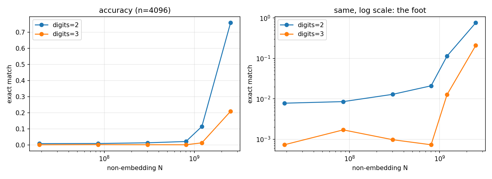
At $n = 256$, $d = 2$ accuracy reads as flat (“zero”) through 1B parameters. At $n = 4096$ the foot resolves into a smooth, above-chance rise: $A = 0.0078,\ 0.0085,\ 0.0129,\ 0.0210$ across 70M–1B (chance is $\sim 0.005$ against the $\sim 180$-value answer space). This directly confirms Schaeffer et al.’s second prediction: small models do not have zero accuracy; they have small accuracy that a small test set censors to zero, since one cannot measure $A \ll 1/m$. The “appears from nothing” reading of such curves is a resolution artifact, exactly as they argued.

The transition’s sharpness is resolution-stable

The same curves end in a steep rise: $0.114 \to 0.759$ between 1.4B and 2.8B. For $d = 2$ the composition mechanism is structurally absent ($\ell = 1$): the macroscopic metric and the microscopic per-token quantity are the same number, and that number itself jumps (mean target-token log-probability $-4.18 \to -0.78$) across the interval. The remaining artifact candidate is test-set resolution, which Experiment 1 addresses directly.

Subsampling at $m = 64, 128, \ldots, 4096$ and extracting

\[s_m = \max_N \frac{dA_m}{d\log N}\]

gives a two-regime answer:

• At the main transition, $s_m$ is flat: $\theta = +0.002$ for $d = 2$ ($+0.001$ to $+0.004$ for $d = 3$) over a 64-fold range in $m$, consistent with zero within bootstrap errors. The maximum slope sits between two accuracies (0.114 and 0.759) that even 64 items resolve; additional statistics neither soften nor sharpen it.
• In the foot (70M–1B window), $s_m$ falls with $m$: from 0.0167 to 0.0082, with a single power-law fit giving $\theta_{\mathrm{foot}} \approx -0.2$. Here low resolution manufactures apparent sharpness and statistics dissolve it — the resolution mechanism again, in quantitative form: the bias is an extreme-value effect with a measurable decay exponent, derived in Appendix A. Foot-region sharpness should not be taken at face value.

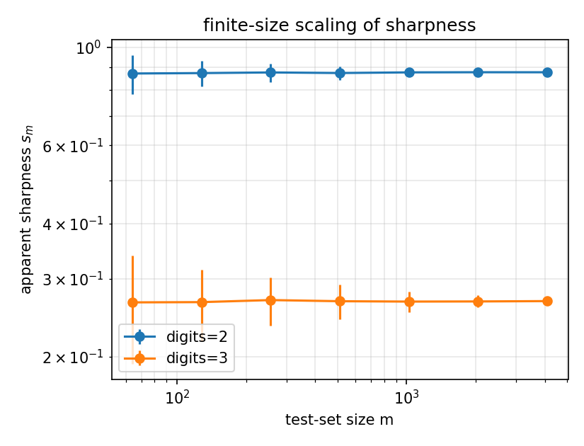
The picture from the two results above is symmetric. Both artifact mechanisms are measurably present where they apply: censoring hides the foot, and finite statistics manufacture sharpness within it. Both are measurably absent at the main transition: composition is structurally unavailable at $\ell = 1$, and the sharpness is invariant under a 64-fold change in resolution. What survives both controls is a property of the underlying per-token quantity, not of the measurement. The honest scope statement: with six sizes, the parameter-scaling transition is localized to one interval and supports “metric-stable and resolution-stable,” not “divergent” — and that statement, about emergence with model scale, is as far as six size points can take it.

The actual emergence test: parameter-axis susceptibility

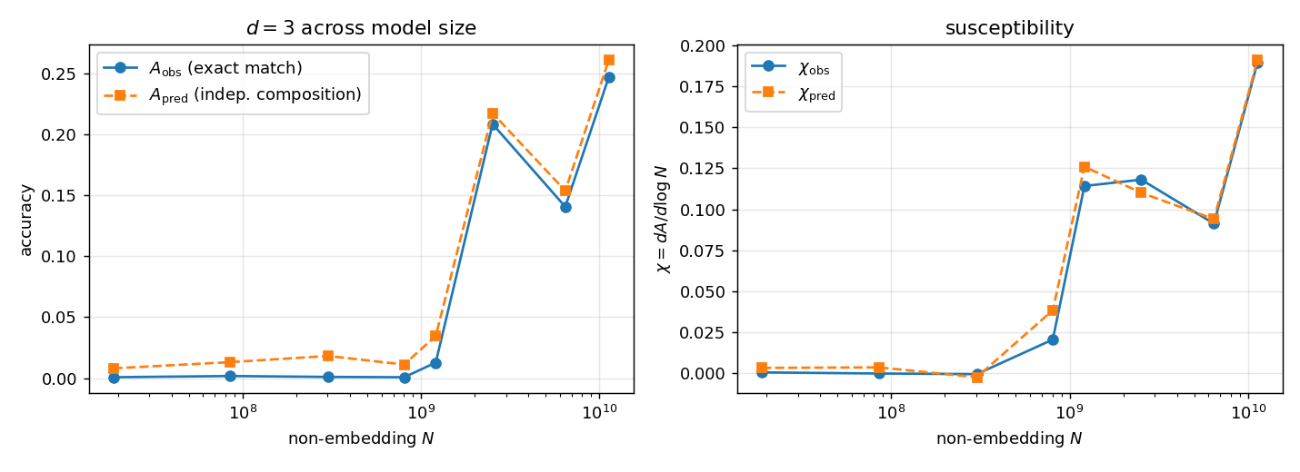
The central question of the post arrives here: is the across-$N$ jump in exact match a real sharpening of what the model knows, or only the discontinuous metric compressing a smoothly-improving per-token quantity? Experiment 1 cleared the two measurement artifacts at $d = 2$, but there the composition mechanism is structurally absent ($\ell = 1$); to put composition itself on trial I move to $d = 3$, where $\ell \approx 1.85$ and exact match is a genuine product of per-token accuracies. The construction is the training-axis test of Part II, transported to the parameter axis: build the observed exact match $A_{\mathrm{obs}}(N)$ and the per-position marginal token accuracies $p_j(N)$; compose the marginals under independence into

\[A_{\mathrm{pred}}(N) = \Big\langle \prod_{j < \ell_i} p_j \Big\rangle_i\]

the exact match a model with those same marginals but independent token errors would post; and compare the two susceptibilities

\[\chi_{\mathrm{obs}} = \frac{dA_{\mathrm{obs}}}{d\log N}\]

and

\[\chi_{\mathrm{pred}} = \frac{dA_{\mathrm{pred}}}{d\log N}\]

across the eight sizes. The small sizes use $n = 4096$ to clear the censoring floor; $6.9$B and $12$B use $n = 1024$.

$N_{\mathrm{ne}}$	$A_{\mathrm{obs}}$	$A_{\mathrm{pred}}$	$p$	$\chi_{\mathrm{obs}}$	$\chi_{\mathrm{pred}}$
$1.9\times10^{7}$ (70M)	0.0007	0.0080	0.038	$0.001$	$0.003$
$8.5\times10^{7}$ (160M)	0.0017	0.0131	0.058	$-0.000$	$0.004$
$3.0\times10^{8}$ (410M)	0.0010	0.0182	0.073	$-0.000$	$-0.002$
$8.1\times10^{8}$ (1B)	0.0007	0.0112	0.055	$0.021$	$0.039$
$1.2\times10^{9}$ (1.4B)	0.0127	0.0346	0.127	$0.114$	$0.126$
$2.5\times10^{9}$ (2.8B)	0.2085	0.2173	0.454	$0.118$	$0.110$
$6.4\times10^{9}$ (6.9B)	0.1406	0.1537	0.381	$0.091$	$0.094$
$1.1\times10^{10}$ (12B)	0.2471	0.2611	0.504	$0.189$	$0.191$

Four observations:

The foot reappears on the parameter axis The four sizes from 70M to 1B sit at $A_{\mathrm{obs}} \approx 0.0007$–$0.0017$ — small and above chance, not zero — while their composed prediction runs $0.008$–$0.018$. The 1B point reads exactly zero at $n = 1024$ and resolves to $0.0007$ only at $n = 4096$: the censoring of the foot, reproduced along $N$ rather than along test-set size.

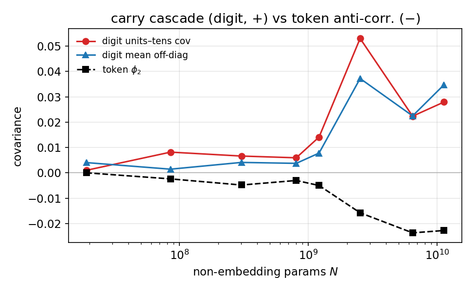
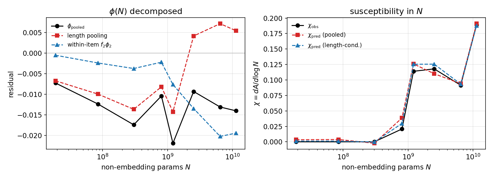
The composition over-predicts at every size, with one sign $A_{\mathrm{pred}}$ exceeds $A_{\mathrm{obs}}$ at all eight sizes — signed gap $+0.007$ to $+0.022$, mean $0.013$, never changing sign. An independence assumption over-counts exact match, so the true joint is harder than the marginals imply: the token-correctness indicators are weakly anti-correlated, not positively correlated. At the token level this looks like localized error — when an answer is wrong it is usually wrong in a single token, so the errors appear to repel rather than cluster. That reading does not survive the dissection: conditioning on the number of output tokens and re-scoring on digits flips the sign, exposing a positive carry cascade at the digit level that the floating BPE boundary disguises as token-level anti-correlation. I work this residual — and the length-pooling artifact hiding inside it — out in full below. This is the same-signed residual found on the training axis in Part II, smaller here than there (where it peaks near $0.03$).

The susceptibilities track; the residual is in the level, not the slope $\chi_{\mathrm{obs}} \approx \chi_{\mathrm{pred}}$ at every size — composition reproduces the shape of the across-$N$ rise. The steep interval is $1.4$B $\to 2.8$B ($A: 0.013 \to 0.21$, $p: 0.13 \to 0.45$). What the metric-composition account captures is how the transition is shaped along $N$; what it misses is a small, uniform, correctly-signed level offset.

Two caveats bound the claim First, a genuine non-monotonicity: $A_{\mathrm{obs}}$ runs $0.21 \to 0.14 \to 0.25$ from 2.8B to 6.9B to 12B, and the dip is present in the per-token accuracy too ($0.45 \to 0.38 \to 0.50$), so it is a real weakness of Pythia-6.9B on this task, not a metric artifact. Second, both susceptibilities peak at the largest size as a one-sided edge difference: the transition is not resolved inside $70$M–$12$B — $A$ is still climbing at 12B — so the peak is unlocated, and a finite-difference $\chi$ over eight uneven points straddling a dip is not a robust estimator of it. The defensible statements are the level of $A$ and the sign of the $A_{\mathrm{pred}} - A_{\mathrm{obs}}$ gap; the peak location is not one of them.

The honest reading is that along the parameter axis, the $d = 3$ transition sits on the same metric-composition rung the training axis identifies — the deflationary account mostly holds with scale, carrying the same small correlated-error residual — but eight uneven Pythia points, with a real 6.9B dip and an unresolved peak, are too coarse for this to stand as an independent confirmation. The obvious objection is that all of this is a property of Pythia, not of the phenomenon. The next section answers that objection directly.

Cross-family replication: does the picture survive a change of family?

The single sharpest objection to everything above is that it is a fact about Pythia — one suite, one corpus (the Pile), one tokenizer, one architecture, with a visible idiosyncrasy (the 6.9B dip) to prove the suite has idiosyncrasies. A composition result that reproduces on an independent family, trained on different data with a different tokenizer, is worth far more than a tighter fit on Pythia alone.

BLOOM is close to the ideal control, for four reasons, only the first of which is obvious:

1. It is not math-tuned BLOOM (2022, the multilingual ROOTS corpus) predates the instruction- and math-saturated pretraining of the current generation. Three-digit addition is genuinely hard for it at small scale, so there is a transition to see; modern suites (Qwen2.5, Llama-3, Gemma-2) ace the task at every size and show no curve at all.
2. It holds the data axis fixed across sizes Every BLOOM size is trained on the same ROOTS corpus and a matched token budget — about $341$ billion tokens — so moving along $N$ changes neither the training distribution nor the training duration. This is the property that makes Pythia a clean $N$-scan, and the one that compute-optimal suites (Cerebras-GPT, anything Chinchilla-scaled) deliberately violate by growing the token count with $N$.
3. It is maximally independent of Pythia Different corpus (ROOTS vs the Pile), different tokenizer (a 250k multilingual vocabulary vs the 50k GPT-NeoX one, hence a different number tokenization and a different $\ell$ — measured at $1.65$ here against Pythia’s $1.85$), different positional scheme (ALiBi vs rotary). If the composition picture survives all of that, it is not a property of any one of those choices.
4. Its non-embedding sizes nearly coincide with Pythia’s This is an accident of BLOOM’s large vocabulary, which inflates the embedding and leaves the non-embedding counts at ${0.30,\, 0.68,\, 1.21,\, 2.36,\, 6.04}\times 10^{9}$ — essentially Pythia’s 410M, 1B, 1.4B, 2.8B, and 6.9B. The comparison is therefore nearly paired: at matched non-embedding $N$ the two families can be read against each other, and in particular BLOOM places a point at $6.0\times10^{9}$, exactly where Pythia-6.9B dips — a direct test of whether that non-monotonicity belongs to the phenomenon or to Pythia.

What BLOOM does not do is densify the transition: in non-embedding units it carries the same $1.2$–$2.4\times10^{9}$ gap Pythia does. This is a robustness-and-independence check, not a finer localization.

The sweep is $d = 3$, 4-shot, BLOOM 560M–3B at $n = 4096$ and 7.1B at $n = 1024$ (offloaded). All five sizes, with the same composition construction:

$N_{\mathrm{ne}}$	$A_{\mathrm{obs}}$	$A_{\mathrm{pred}}$	$p$	gap
$3.0\times10^{8}$ (560M)	0.0015	0.0234	0.052	$+0.022$
$6.8\times10^{8}$ (1.1B)	0.0002	0.0266	0.060	$+0.026$
$1.2\times10^{9}$ (1.7B)	0.0007	0.0306	0.064	$+0.030$
$2.4\times10^{9}$ (3B)	0.0017	0.0358	0.074	$+0.034$
$6.0\times10^{9}$ (7.1B)	0.0029	0.0455	0.094	$+0.043$

Two things reproduce; one differs, and the difference is the point.

The foot of the accuracy curve reproduces, on a corpus and tokenizer that share nothing with the Pile Every BLOOM size from 560M to 7.1B sits at a small, censored $A_{\mathrm{obs}}$ (0.0002–0.0029) over above-zero per-token accuracy ($p = 0.05$–$0.09$), with a positive composition gap throughout. The censoring-of-the-foot mechanism is not a Pythia artifact.

The composition over-predicts with the same sign $A_{\mathrm{pred}} > A_{\mathrm{obs}}$ at all five sizes, as in Pythia. One honest qualification is that in the foot this gap is dominated by the censoring of $A_{\mathrm{obs}}$ near zero, not by a clean correlated-error residual at resolved accuracy — the latter is what Pythia’s 2.8B–12B points demonstrate ($+0.009$ to $+0.014$ at $A \sim 0.2$–$0.5$), and BLOOM has not reached resolved accuracy within its released range. So BLOOM confirms the sign of the composition bias; it does not yet independently pin its magnitude at resolved $A$.

The transition sits roughly an order of magnitude later in $N$ This is the substantive cross-family difference. At matched non-embedding $N$, Pythia has already climbed where BLOOM is still in the foot: at $1.2\times10^{9}$, Pythia-1.4B reads $p = 0.13,\ A = 0.013$ against BLOOM-1.7B’s $p = 0.064,\ A = 0.0007$; at $\sim!2.4\times10^{9}$, Pythia-2.8B has reached $A = 0.21$ while BLOOM-3B is still at $A = 0.0017,\ p = 0.074$. BLOOM’s per-token accuracy merely increases from $0.052 \to 0.074$ over the same decade in which Pythia’s runs $0.073 \to 0.454$. Three-digit addition emerges about a decade of $N$ later for BLOOM, which is unsurprising for a multilingual ROOTS model measured against the English-dense, arithmetic-rich Pile.

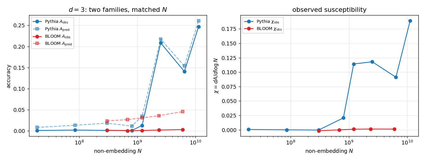
The reading is that the deflationary mechanism — the foot, the censoring, the positive composition bias — is not a property of Pythia. It reappears in a family that shares almost nothing with Pythia but its non-embedding parameter count. What is family-dependent is the transition’s location: BLOOM places it beyond the reach of its released small models, so the cross-family check vindicates the mechanism while declining to independently resolve the steep transition. BLOOM-7.1B, at $N = 6.0\times10^{9}$ and matched to Pythia-6.9B, makes the point concrete: it reads $A_{\mathrm{obs}} = 0.003$, $p = 0.094$ — still in the foot. BLOOM has not emerged anywhere in its released range, so the dip-adjudication is moot here: there is no risen accuracy at which a dip could appear.

Beyond independence: does the correlation reorganize at the transition?

A metric artifact and a genuine collective transition can look identical in the marginals; they need not look identical in the correlations. Independence is a mean-field step — it multiplies the per-position accuracies and discards the connected correlation — so if anything escapes the deflationary account, this is where it hides: in the structure the composition throws away, not in the $p_j$ it keeps. The residual is small, but its sign is a measurement. Within the two-token answers (and at $d=3$ the answer is one or two tokens, never more),

\[A_{\mathrm{obs}} - A_{\mathrm{pred}} = \mathrm{Cov}(c_1,c_2)\]

exactly, with no higher cumulant: the residual is that discarded correlation. I consider two things — what sign it takes, and whether its structure changes across the transition, since a genuine collective reorganization would manifest itself as this correlation swelling at the critical $N$, exactly where the marginals (all independence can see) show nothing. Per size:

size	$\phi(c_1,c_2)$	$P(c_2{=}1\mid c_1{=}0)$	$P(c_2{=}1\mid c_1{=}1)$	$p_2$	single-slip
1.4B	$-0.079$	0.117	0.051	0.11	26%
2.8B	$-0.069$	0.623	0.550	0.60	69%
6.9B	$-0.111$	0.554	0.425	0.52	62%
12B	$-0.102$	0.703	0.603	0.67	76%

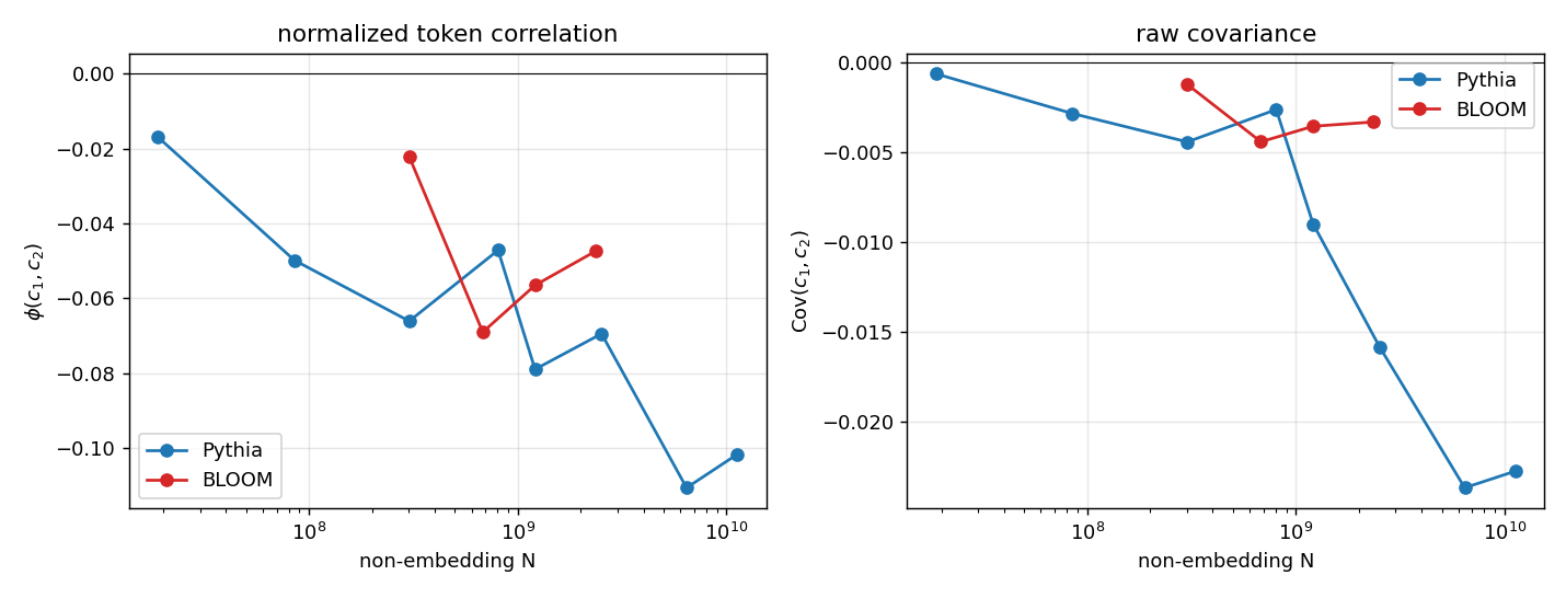
The token errors are weakly anti-correlated — but the sign is the tokenizer’s, not the model’s $\phi$ is negative at all eight sizes. At 12B, knowing the first token is wrong raises the second’s hit rate to $0.70$ — above its $0.67$ marginal — while knowing the first is right drops it to $0.60$. Taken at face value this reads as localized error, failures concentrating in the harder high-order first token ($p_1 < p_2$ at every size; at 12B “first wrong, second right” outnumbers “first right, second wrong” $403$ to $120$). But the token is the wrong unit. Conditioning the covariance on (answer length, token split) collapses it almost to zero, and re-scoring on the digit alphabet flips the sign: the per-digit error covariance is positive, largest for the adjacent units–tens pair. This is a carry cascade: place-value addition propagates a carry from each digit into the next, so an error at one place corrupts the place above it, and positive correlation between adjacent-digit errors is the signature any carry-respecting algorithm must produce. The token-level $\phi$ is the wrong quantity to interpret — its negative sign is only what that cascade looks like after the floating BPE boundary pools over heterogeneous digit partitions. The mechanism is worked out in full on the training axis in Part II, where conditioning kills $85\%$ of the token covariance and the digit-level units–tens coupling grows to $+0.06$ through training; the same correction applies here, size for size. Mechanistically, the model adds place by place with carry propagation, its errors riding the carry chain; the apparent single-token localization is the tokenizer’s signature, not the model’s algorithm.

The correlation does not reorganize at the transition This is the emergence-relevant result. $\phi(N)$ runs $-0.02,\,-0.05,\,-0.07,\,-0.05,\, -0.08,\,-0.07,\,-0.11,\,-0.10$ across the eight sizes: small, negative, drifting only slightly, with no peak or sign-change through the steep interval ($1.4$B$\,\to\,2.8$B: $-0.079 \to -0.069$). To the resolution of eight points, the correlation independence throws away is scale-stable — it does not swell at the transition the way a critical susceptibility would. The failure mode appears to reorganize — single-token failures climb from $8\%$ to $76\%$ across the rise — but that is the marginals moving: as $p_1,p_2$ rise, single-token failures must come to dominate both-wrong even under independence, and $\phi$, which divides that out, stays flat. The defensible statement is “failures appear to localize as accuracy rises,” not “the model reorganizes into a localized-error regime at the transition.”

Most of the accuracy foot’s over-prediction is a pooling artifact, not correlation The pooled first-token marginal mixes the easy one-token answers with the first token of two-token answers; splitting the gap into that pooling effect plus the genuine two-token covariance separates them. In the foot the gap is almost all pooling — the one-token answers (merged four-digit numbers like “ 1935”) are never correct there, so the pooled marginal over-credits them — and the covariance is negligible. At the plateau the pooling term reverses and the covariance takes over: at 12B the net gap $+0.014$ is a token-covariance term $+0.019$ against pooling terms summing to $-0.005$. So the anti-correlation is real where accuracy can resolve it, and the foot gap should not be read as correlation at all.

What this says about the mirage Independence is analogous to a mean-field step — multiply the marginals, discard the connected correlation — and recovering that correlation does not rescue real emergence; it deepens the deflationary reading. The sign means the exact-match readout is, if anything, slightly more suppressed than independence assumes, so $p^{\ell}$ understates the apparent sharpness rather than inventing it. However, the flatness means the discarded object carries no transition of its own. The one place genuine collective behavior could have hidden from the marginals — a correlation that diverges at the critical $N$ — is, to this resolution, simply not there. BLOOM shows the same negative $\phi$ across its foot ($-0.02$ to $-0.07$), so the sign is not a Pythia artifact.

The emergence claim of Wei and Schaeffer is intrinsically about the parameter axis: an ability is “emergent” if it is absent in small models and present in large ones, which one can only assess by comparing different models of different sizes — exactly what the susceptibility test above does. Part II turns to the training axis instead, tracing a single fixed-size model through its checkpoints. That is no longer a statement about emergence-with-scale; it is a test of the metric-composition mechanism itself — how per-token accuracies multiply into a sequence-level metric, true or false independently of which axis one moves along — and it buys the dense coverage in a single control variable that eight size points here cannot.

Discussion: emergence with model size

Putting the pieces together along the parameter axis, the per-token marginals $p_j(N)$ are smooth across the eight Pythia sizes; the exact-match curve is sharp; and the composition law, which simply multiplies those smooth marginals, recovers most of that sharpness on its own. What it misses is small and has a definite sign: the connected correlation $\phi(N)$ is a few percent, negative, and flat through the steep interval, with no peak where a critical susceptibility would diverge. The one object that could have carried a genuine transition past the smooth marginals is, to the resolution of eight sizes, simply not there. That value is token-level, though, and Part II shows the token-level $d = 3$ residual to carry an answer-length pooling artifact that flips its sign; $\phi(N)$ here inherits the same caveat, with the digit-level read — which turns the residual into a small positive carry cascade — feasible only on the dense training axis.

So for $d = 3$ the across-$N$ transition sits on the metric-stable rung: the apparent emergence is a hard metric composing smooth per-token competence, plus a small residual that is mostly tokenization pooling over a smooth, positive digit-level carry cascade — real, but analytic in $N$. By the strict, finite-size-scaling reading of emergence this is a negative result — no qualitative change of state with scale — and it is a quantitative negative, not a failure to find one: the would-be order parameter is measured, and it does not move. Whether the same holds along the training axis — where the correlation is concrete (carry propagation), the checkpoint coverage is dense, and the loss-perspective reading of emergence (Du et al. (2024)) can be met head-on by mapping accuracy onto the loss curve — is the question of Part II.

Where the analogy breaks

Phase transitions have an order parameter tied to spontaneous symmetry breaking; LLM capabilities have no obvious one. Critical behavior requires a thermodynamic limit; LLM scaling is always finite, and the “sizes” being scaled — parameters, data, test items — are not a single $L$. The analogy licenses a methodology, measuring how signatures scale with resolution; it does not license a structural identification, and nothing above should be read as a claim that language models are near-critical systems.

Part II makes the dictionary behind this methodology explicit for the training axis — the loss as the free energy, the accuracy as the order parameter, and the distinction between the response susceptibility $dA/d\log D$, which peaks for any sigmoid, and the fluctuation susceptibility that alone diverges at a continuous transition — and uses it to meet the loss-perspective reading of emergence head-on.

Appendix A: count statistics of the sharpness estimator

The accuracy foot’s $\theta_{\mathrm{foot}} \approx -0.2$ from a single power-law fit hides cleaner structure. Decomposing $s_m = s_\infty + \delta_m$, the full-set value is $s_\infty = 0.0082$ and the excess $\delta_m$ falls as a power law with exponent $\alpha \approx 0.8$–$1.0$ over $m = 64$–$1024$ before vanishing into the plateau; the shallow $-0.2$ is what a single power law fitted across the plateau-contaminated range produces.

The exponent is diagnostic of the noise regime, and the controlling parameter is the expected success count $\lambda = mA$, not $m$. The estimator $s_m$ takes a maximum over intervals of (true slope $+$ fluctuation), and the maximum of fluctuating quantities is biased upward — finite test sets manufacture sharpness wherever the curve is noisy. In the Gaussian regime, $\lambda \gg 1$, accuracy fluctuations scale as $\sqrt{A/m}$ and the bias decays with $\alpha = 1/2$. In the count regime, $\lambda \lesssim O(10)$, a fluctuation is one discrete extra success moving $\hat{A}$ by exactly $1/m$, and the bias decays with $\alpha \approx 1$. With $A \sim 10^{-2}$ in the foot, the crossover $\lambda \sim 1$ sits near $m \sim 10^2$ and the Gaussian regime arrives only at $m \sim 10^3$ — where the excess has already vanished. The measured $\alpha \approx 0.8$–$1.0$ is the count-regime exponent with the expected crossover.

The two decay rates follow from one calculation. The estimator

\[s_m = \max_i (\beta_i + \xi_i)\]

maximizes over $K$ adjacent intervals, each carrying the true slope $\beta_{i}$ plus a mean-zero fluctuation $\xi_{i}$ of scale $\sigma_m$; the upward bias is

\[\mathbb{E}[\max_i \xi_i] \sim c_K\,\sigma_m\]

with $c_K$ a slowly varying ($\sqrt{\log K}$) order-unity factor. Everything is in how $\sigma_m$, the standard deviation of the slope estimate, scales with $m$. The slope is a finite difference of accuracies

\[\hat A = (1/m)\sum \mathbf{1}[\text{success}]\]

so $\sigma_m \propto \mathrm{sd}(\hat A)$.

In the Gaussian regime ($\lambda = mA \gg 1$) the success count $\sum_i \mathbf{1}[\text{success}_i]$ is a sum of $m$ i.i.d. Bernoulli($A$) indicators, so by the central limit theorem it is asymptotically $\mathcal{N}!\big(mA,\, mA(1-A)\big)$ and the binomial gives

\[\mathrm{sd}(\hat A) = \sqrt{A(1-A)/m} \sim m^{-1/2}\]

hence

\(\delta_m \sim m^{-1/2}\) and \(\alpha = \tfrac12\).

In the count regime ($\lambda \lesssim 1$) the central limit theorem has not yet taken hold — for rare events its approach to the Gaussian is governed by the expected count $\lambda$, not by $m$ — so successes are still Poisson with mean $\lambda = mA$, and the slope estimate is quantized: each additional success moves $\hat A$ by exactly $1/m$, so the smallest non-zero fluctuation — and hence the bias floor of the maximum — is of order $1/m$ itself. The upward bias therefore tracks $\sigma_m \sim 1/m$, giving $\delta_m \sim m^{-1}$ and $\alpha = 1$. The crossover between the two is at $\lambda \sim 1$, i.e. $m \sim 1/A$, exactly where the data turn over.

The practical moral: a 4096-item benchmark sounds large, but for a task at 1% accuracy it holds $\sim 40$ successes. The statistics of capability feet are count statistics at any test-set size in common use, and error analysis of emergence claims is naturally done in $\lambda = mA$, not $m$.

Reproducibility

All experiments run on a single Apple M3 Pro chip — an Arm system-on-chip with a 12-core CPU (6 performance + 6 efficiency cores) and an 18-core integrated GPU sharing 18 GB of unified memory, with PyTorch on the Metal Performance Shaders (MPS) backend rather than CUDA. All evaluations are fp16, and the unified-memory budget sets where offloading becomes necessary rather than a hard ceiling: the 70M–2.8B models fit in the 18 GB and run on the GPU directly, 6.9B still fits in fp16, and 12B exceeds the budget and is run in fp16 with CPU offload (device_map=auto) — slower, but enough to evaluate it at all. Task generators, evaluation code, sweep configurations, and the analysis producing every number and figure above are in scaling-experiments, with the executed analysis notebook alongside.

---

Prose edited with the assistance of Claude (Anthropic), which also checked the numbers against the analysis artifacts and ran supplementary experiments. I ran the main experiments and vouch for every claim here.