Introduction

In Part I, I studied a benchmark’s accuracy as a function of parameter count $N$ using eight Pythia models of increasing size, each scored at the end of training and asked whether the sharp increase in accuracy survives a finite-size-scaling analysis in the number of model parameters $N$. This post runs the same kind of analysis on the training-data axis: I select a single model at fixed parameter count $N$ and record how both the per-token error rate and the benchmark built from it evolve as a function of $D$, the number of tokens seen.

Wei et al. (2022) did not discuss training-set size in their emergence story, since most model families fix the number of training tokens across sizes. As a result, the emergence debate has mostly played out along scale. In Schaeffer, Miranda & Koyejo (2023), the authors made the following statement about composition: a smooth per-token accuracy $p$, pushed through a hard sequence-level metric, gives $A \approx p^{\ell}$, and that product turns a featureless underlying curve into a sharp one. As arithmetic this is indifferent to how the given value of $p$ evolves, but the evidence for it is read off model scale, where per-token loss falls as a power law in parameters and compute. In this post, I look at the training-dynamics of a single model and analyze how the sequence-level metric is assembled out of per-token competence. Specifically I ask: how far do the per-token errors entering the composition deviate from complete independence? The composition law $A \approx \prod_j p_j$ assumes the per-token errors are independent across answer positions. This assumption can be directly probed from the data. So along training I follow two quantities: the per-token error rate $1 - p(D)$ as it falls over the training run, and the correlation between those errors across positions. Specifically I consider the gap between the product of the marginals and the observed joint accuracy as a measure of the deviation from independence.

In this post I examine whether the benchmark’s sharp turn-on is a transition or an artifact of the metric, along the training axis for a single model held fixed and the token budget $D$ swept across checkpoints, so that accuracy and loss can be tracked together along one trajectory. Rather than looking at the peak in the response $\chi = dA/d\log D$ as the signature of a transition, I will look at the behavior of the fluctuation susceptibility and the correlation length under finite-size scaling, i.e. the criterion that actually classifies a transition. I find that composition, $A \approx p^{\ell}$, accounts for essentially all of the steepness. The only genuine error correlation is a small, positive, short-ranged carry cascade, visible at the digit level and opposite in sign to the negative token-level correlation a naive null reports; and that the connected correlation stays small and non-diverging through the peak. Along the way I reconcile the deflationary reading with the loss-perspective account of Du et al. (2024), mapping accuracy directly onto pre-training loss and finding the response peak to sit on a smooth, monotone stretch of the loss curve. I conclude that along this axis, on this task, the turn-on is a crossover — smooth competence read through a hard metric — not a transition of any order.

Code and executed notebooks: scaling-experiments.

The composition mechanism, and what the training axis adds

For exact match on a length-$\ell$ target a smooth per-token accuracy $p$ composes to

\[A \approx p^{\ell}\]

which rises abruptly even when $p$ is a featureless power law. Rescoring the BIG-Bench catalogue with locally linear metrics — token edit distance, Brier score — dissolves most of the emergence. This fixes the full shape of the sharpening of the accuracy curve, given $p$.

In Part I, I looked at this quantity for models of different parameter counts. Two things open up once the model is held fixed and one considers the training axis. The first is resolution. For one model one can obtain a dense grid of checkpoints through training which is fine enough to measure a susceptibility in seen tokens $D$ defined as

\[\chi = \frac{dA}{d\log D}\]

By contrast, for model parameters $N$ there are only a few coarse points on the same curve. The second is a check on the assumption in $A \approx \prod_j p_j$ that the per-token errors are independent across positions. Composition fixes the joint exact-match exactly, given the marginals, so the gap between that prediction and the measured joint accuracy is the deviation from independence — a connected correlation for multi-token answers, but only when the marginals are not also pooling over heterogeneous items, as the results below make concrete.

Setup

The model suite, the synthetic few-shot $d$-digit addition task, the readout, and the baselines are exactly as in Part I; I consider the same two measured quantities — teacher-forced per-token accuracy $p$ and exact match $A$, with the teacher-forced/free-running equivalence used as a computational shortcut — as is the $d = 2$ tokenizer coincidence that gives $\ell = 1$ and $A = p$ identically (composition structurally absent), against $d = 3$ with $\ell \approx 1.85$ (one- or two-token answers, composition nontrivial).

From the parameter axis to the training axis Part I scored each Pythia size once, at the end of training, and scaled the parameter count $N$. Here I hold the model size fixed and scale $D$, the number of tokens seen, using the 154 public intermediate checkpoints released for every size. The batch schedule is identical across sizes, so checkpoint step $t$ corresponds to a fixed token count ($D \approx 2.1\times10^{6}\,t$) and the checkpoint index is a clean proxy for $D$. The sweep below walks a single fixed-size model through 11 log-spaced checkpoints — the dense $D$-coverage a handful of model sizes cannot give — which is what lets me measure a susceptibility $\chi = dA/d\log D$ in seen tokens, rather than the coarse finite difference in $N$ that Part I was limited to.

A checkpoint-integrity caveat The training axis needs checkpoints whose weights genuinely differ, and pythia-2.8b fails that test: its Hub intermediate checkpoints serve the final-step weights at every revision, identical to the bit by weight checksum. I therefore verify each model by checksum before use and run the sweep on pythia-2.8b-deduped, which passes (distinct, monotonically evolving checksums).

Experiment: susceptibility along training

The susceptibility test I fit the smooth microscopic quantity $p(D)$ from the well-resolved regime — $D$ being the number of tokens seen at fixed model size — compose it through the per-item target lengths to obtain $A_{\mathrm{pred}}(D)$, and compare

\[\chi_{\mathrm{pred}} = \frac{dA_{\mathrm{pred}}}{d\log D}\]

against $\chi_{\mathrm{obs}}$: peak location, height, and shape. Agreement means the composition mechanism suffices for this task and the errors can be treated as independent; any discrepancy represents a deviation from that assumption. The composition law assumes teacher forcing, so I record both teacher-forced and free-running accuracies and report their gap.

Results

Susceptibility test along the training axis

To test the composition mechanism as a function of $D$ I take a single fixed-size model (pythia-2.8b-deduped, per the integrity check in the setup) evaluated at $11$ log-spaced checkpoints, which walks through its training transition densely enough to measure a response function. This is a transition in one model as it learns, not a comparison across model scales — so it speaks to how the sequence-level metric is built from per-token accuracies, not to emergence with parameters.

On $d = 2$ the model traces a full sigmoid over training, $A = 0 \to 0.85$, with the steep rise between $D \approx 7\times10^{10}$ and $1.3\times10^{11}$ tokens. Since $d = 2$ has $\ell = 1$, this curve is the per-token accuracy $p(D)$ — what the figure shows is the per-token error rate $1 - p(D)$ falling over training, with no metric standing between the microscopic quantity and the benchmark. The susceptibility $\chi = dA/d\log D$ has a clean peak of $0.535$ at $D = 1.3\times10^{11}$ — a clean response peak, measured along training rather than asserted. A response peak alone is not a transition; every sigmoid has one, and what a genuine transition would additionally require is set out in the discussion.

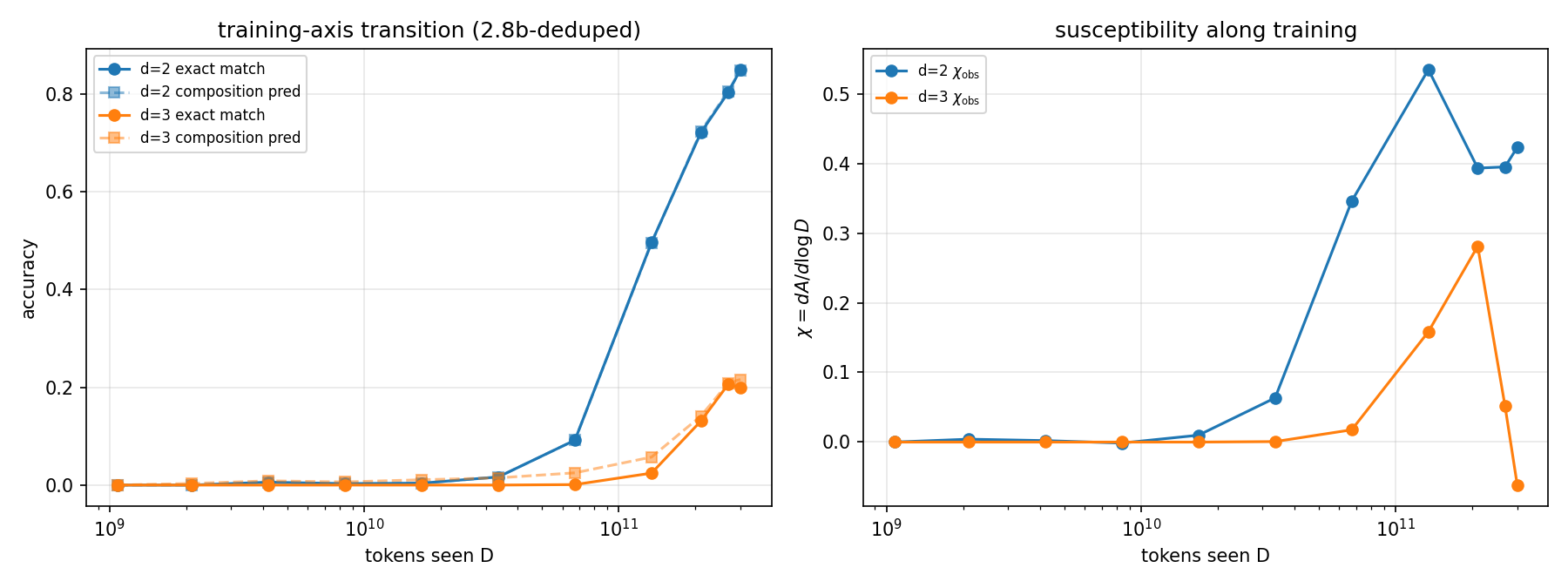
Because $d = 2$ has $\ell = 1$, the composition model’s prediction $A_{\mathrm{pred}} = \prod_j p_j$ reduces to $p$ itself, and indeed $A_{\mathrm{pred}}$ and $A_{\mathrm{obs}}$ agree to machine precision at every checkpoint, with $\chi_{\mathrm{pred}}$ peaking at $0.539$ against $\chi_{\mathrm{obs}} = 0.535$ which is shown by the same peak, in the same place. This is the consistency check: where composition is trivially exact, it is exactly exact.

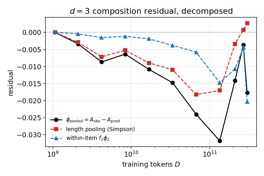
For $d = 3$ the answer runs to $\ell \approx 1.85$ tokens on average and composition is non-trivial. A clean directional gap opens: the independence prediction overpredicts the observed joint at every checkpoint with signal, and the connected residual $\phi \equiv A_{\mathrm{obs}} - A_{\mathrm{pred}}$ is negative, peaking at $\phi = -0.032$ in the steep part of the rise ($A_{\mathrm{pred}} = 0.057$ against $A_{\mathrm{obs}} = 0.025$ at $D = 1.34\times10^{11}$). The fast reading is that this is the failure of the independence assumption, with the sign saying per-token correctness is anti-correlated. That reading is too fast — most of the residual is not a correlation at all. The rest of this section takes it apart, and what is left is the opposite sign.

The residual is mostly two answer-length classes, pooled

The NeoX tokenizer assigns a single token to integers up to three digits, so the $d = 3$ test set is really two answer-length classes: three-digit sums ($\ell = 1$, one token) and four-digit sums ($\ell = 2$, two tokens), with fractions $f_1 = 0.15$, $f_2 = 0.85$ at the residual peak. The pooled null estimates one position-0 marginal across both classes and multiplies — and that pooling has an exact cost. Writing $a_S$ for the single-token accuracy, $b_1, b_2$ for the two-token leading/trailing accuracies, and $\phi_2 = \mathrm{Cov}(C_1,C_2)$ for the genuine within-item covariance, the residual factorizes:

\[\phi_{\mathrm{pooled}} = \underbrace{f_1 f_2\,(1-b_2)\,(a_S - b_1)}_{\text{length pooling (Simpson)}} \;+\; \underbrace{f_2\,\phi_2}_{\text{genuine within-item}} .\]

The first term is not an error correlation at all — it is a Simpson effect from mixing two populations of different per-token difficulty. And they differ sharply: at the peak $a_S = 0.054$ but $b_1 = 0.219$. Producing an entire three-digit answer as one token (one draw from $\sim 800$ values) is four times harder than producing the leading token of a four-digit answer, whose value is nearly pinned. With $a_S \ll b_1$ the pooling term is large and negative; it dominates early and decays as the two accuracies equalize over training:

$D$	$\phi_{\mathrm{pooled}}$	pooling	within $f_2\phi_2$	$\phi_2\pm\mathrm{se}$
$1.7\times10^{10}$	$-0.011$	$-0.009$	$-0.002$	$-0.002\pm.001$
$6.7\times10^{10}$	$-0.024$	$-0.018$	$-0.006$	$-0.007\pm.001$
$1.3\times10^{11}$	$-0.032$	$-0.017$	$-0.015$	$-0.017\pm.004$
$2.1\times10^{11}$	$-0.014$	$-0.003$	$-0.011$	$-0.013\pm.007$
$3.0\times10^{11}$	$-0.018$	$+0.003$	$-0.020$	$-0.024\pm.008$

Conditioning the null on length, and the sharpness claim

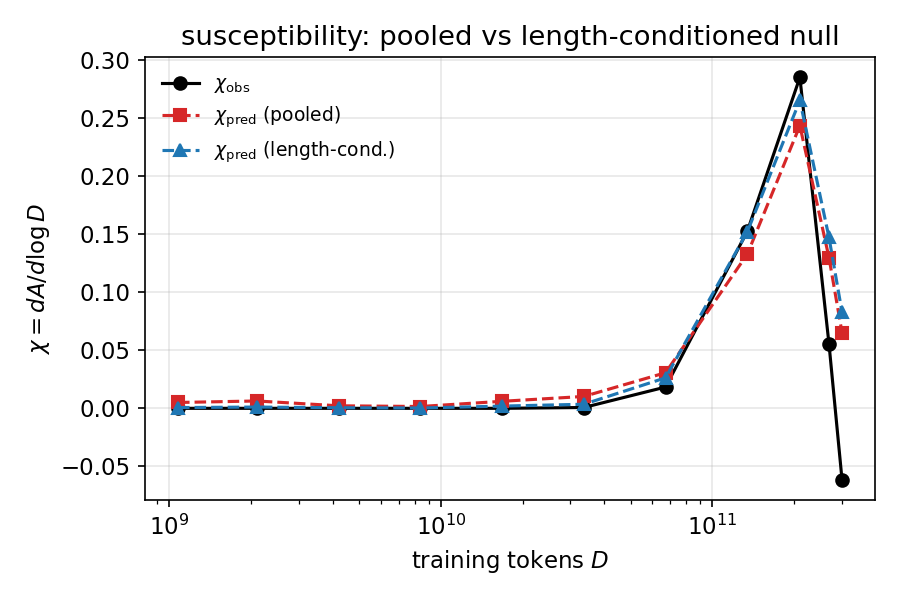
The fix is to condition the null on answer length — compose within each class and recombine, $A_{\mathrm{pred}}^{\mathrm{lc}} = f_1 a_S + f_2 b_1 b_2$ — so the Simpson term is removed by construction and the residual is exactly $f_2\phi_2$. This shifts the susceptibility comparison the test turns on. With one finite-difference estimator throughout ($\chi = dA/d\log D$ on the 11-point log-$D$ grid, $\chi_{\mathrm{obs}} = 0.285$):

null	peak $\chi_{\mathrm{pred}}$	$\chi_{\mathrm{obs}} - \chi_{\mathrm{pred}}$
pooled	$0.243$	$+0.042$
length-conditioned	$0.265$	$+0.020$

Roughly half of the apparent excess sharpness was the pooling artifact: removing it lifts the predicted susceptibility from $0.243$ to $0.265$, and the surviving margin of $+0.020$, on eleven coarse checkpoints with a slightly non-monotone tail, sits within finite-difference noise. So the strong reading I was tempted by — the transition is sharper than composition predicts — does not survive. What survives is the level statement: even length-conditioned, composition overpredicts the joint, because $\phi_2$ is genuinely negative ($-0.017 \pm 0.0044$, $3.9\sigma$ at the peak). Whether that is a correlation is the last question.

The carry cascade is real — at the digit level

First, what a carry cascade is and why it is the error structure to expect. Addition is computed place by place, a carry propagating from each column into the one above whenever the column sums to ten or more. Any procedure that respects place value couples adjacent digits: a wrong digit, or a mishandled carry, at one place corrupts the place above it. The signature such an algorithm must produce is a positive correlation between adjacent-digit errors, concentrated where carries originate (units–tens) — so given that the model emits the answer as a digit sequence, this is the structure to expect a priori if it is doing arithmetic at all; a negative correlation would be the anomaly. That is why the token-level $\phi_2$ below, though negative, is the wrong quantity to interpret: the unit it is computed on is the tokenizer’s, not the place-value alphabet’s.

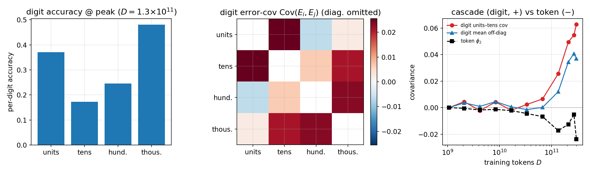
$\phi_2$ is a covariance between two tokens, and the token boundary floats: among four-digit answers the first token holds ${1,2,3,4}$ digits with counts ${11, 385, 202, 17}$. To see the arithmetic instead of the tokenizer, I re-score the residual-peak checkpoint ($D = 1.34\times10^{11}$) and read out each answer digit, right-aligned by place value. The per-place error covariance is positive almost everywhere (units…thousands):

\[\mathrm{Cov}(E_i, E_j) = \begin{pmatrix} \cdot & {+}.026 & {-}.006 & {+}.002\\ {+}.026 & \cdot & {+}.006 & {+}.021\\ {-}.006 & {+}.006 & \cdot & {+}.023\\ {+}.002 & {+}.021 & {+}.023 & \cdot \end{pmatrix},\qquad \overline{\text{off-diag}} = +0.012,\]

with the adjacent units–tens pair — where a mishandled carry actually propagates — the largest entry at $+0.026$. Per-place accuracy runs $[0.37, 0.17, 0.25, 0.48]$ from units to thousands: the units digit needs no incoming carry and is the easiest low place, the carry-laden middle is hardest, and the thousands digit (almost always $1$) is easiest of all. This is the carry cascade the metric-artifact story always implied — positive error correlation, errors clustering across digit positions.

The token-level sign is the opposite only because the floating split pools over heterogeneous partitions. Conditioning $\phi_2$ on (answer length, split point) collapses it almost entirely:

answer digits, split $m$	$n$	token cov
3, split 1	277	$+0.006$
4, split 2	385	$-0.010$
4, split 3	202	$\;\,0.000$
weighted within-group	864	$-0.003$
pooled $\phi_2$	875	$-0.017$

Eighty-five percent of $\phi_2$ is between-group pooling; the genuine within-(length, split) token correlation is $-0.003$, indistinguishable from zero and sign-mixed across groups. With positive digit correlation a fixed partition gives a non-negative token covariance, so the negative $\phi_2$ is not the model’s errors anti-correlating — it is the BPE boundary, floating against the place-value structure, mixing populations one more time.

Run across all eleven checkpoints, the digit-level cascade is not a peak artifact but a feature that grows with training: the units–tens covariance climbs through the transition, from noise to $+0.026$ at the residual peak and on to $+0.063$ by the end of training, exactly as the model consolidates the carry algorithm — while the token-level $\phi_2$ stays negative at every checkpoint. Read mechanistically, that growth is what it means for the model to be adding: competence organized per digit and place, the residual error riding the carry chain — units into tens most strongly, the carry-laden middle places failing together — rather than distributed holistically over the answer or localized to single tokens.

Discussion

Stripped of artifacts, the $d = 3$ training axis says something simple. The metric-composition mechanism accounts for essentially all of the sequence-level sharpness on this task: a smooth per-digit competence, pushed through a hard exact-match metric, manufactures the steep benchmark curve, exactly as the deflationary account argues. The one piece of genuine correlation structure is the carry cascade, and it is positive — visible only when the residual is computed on the place-value alphabet rather than the tokenizer’s. Everything negative in the token-level residual is pooling: first over answer-length classes ($\ell \in {1,2}$, the Simpson term that was half the peak gap), then, inside the two-token class, over the floating token split (most of the rest). There is no anti-correlation to explain. There is a carry cascade, plus two layers of tokenization bookkeeping that disguise it and flip its sign.

That is the cautionary point worth keeping, and the reason the analysis is here in full rather than compressed to its conclusion. The connected residual $A_{\mathrm{obs}} - A_{\mathrm{pred}}$ is a tempting order parameter — it is exactly the deviation from independence — but its sign and magnitude are contaminated by any heterogeneity the null pools over. Answer length and tokenization split are two such axes, and on this task they dominate the genuine signal and even reverse it. A composition test is only trustworthy after conditioning on whatever the marginals are pooled across, or — cleaner — scored at the task-natural granularity, here the digit. The lesson inverts the Dyck-$(k,m)$ post: there the structure lived in correlations invisible to any single per-position statistic; here a per-position null invents structure that the finer description dissolves.

The phase-transition dictionary, made explicit. The rest of this discussion leans on the critical-phenomena analogy, and emergence is the place where it is easiest to overclaim, so it is worth fixing the dictionary together with the one fact it makes unavoidable: here the free energy is the loss, and continuity of the free energy classifies nothing. A first-order transition, a second-order transition, and a smooth crossover all have a continuous free energy; at any finite system size none of them has a true singularity at all. The loss $L(D)$ — a per-token cross-entropy, an averaged negative log-likelihood, the free-energy density of the model’s predictive distribution — is smooth and monotone in $D$, and that smoothness is shared by every case, a genuine transition included. It is not, on its own, evidence that nothing is happening.

The order parameter is the accuracy $A$, the mean of a ${0,1}$ correctness indicator, in the role of a magnetization $m = \langle s \rangle$. This buys one clean statement and withholds another. A first-order transition is a discontinuous jump in the order parameter, and $A$ rises continuously, so nothing here is first-order-like. But a continuous order parameter is equally consistent with a second-order transition and with a crossover, so continuity alone settles nothing. The Part I caveat also still holds: $A$ is tied to no broken symmetry and is not $\partial L/\partial h$ for any field $h$ — this is an analogy of role, not an identity.

The susceptibility is two objects, and only one diagnoses criticality. What this post measures, $\chi = dA/d\log D$, is a response — how fast the order parameter turns on as the control $\log D$ is dialed — and a response peak is generic: every sigmoid has one, so its peak marks the steepest part of the turn-on and nothing more. The susceptibility that actually diverges at a continuous transition is a different object, the fluctuation susceptibility $\chi_{\mathrm{fl}} \propto \sum_{ij}\phi_{ij}$ — the variance of the order parameter, the integrated connected correlation (here the digit-level error covariance), tied by fluctuation–dissipation to a correlation length and divergent only because correlations grow long-ranged. What would separate a genuine second-order transition from composition dressing a smooth curve is therefore not a sharper response peak, which is free, but the fluctuation susceptibility growing without bound: $\phi$ acquiring a range that grows with system size, and the response peak sharpening and rising toward a divergence under finite-size scaling with definite exponents. The discriminator is the singularity structure of the derivatives as the system grows, never the continuity of the free energy. Held to that standard the rise here is a crossover: the genuine connected correlation is small and short-ranged — nearest-neighbor carry coupling, no growth in range — and the response peak is finite.

The loss-perspective rebuttal. The strongest counter to the deflationary reading is not Schaeffer’s but Du et al. (2024), who argue emergence is real once accuracy is plotted against pre-training loss rather than size or compute, and that the loss threshold survives even under continuous metrics. Nothing here conflicts with it, and with the dictionary above the reconciliation is immediate. 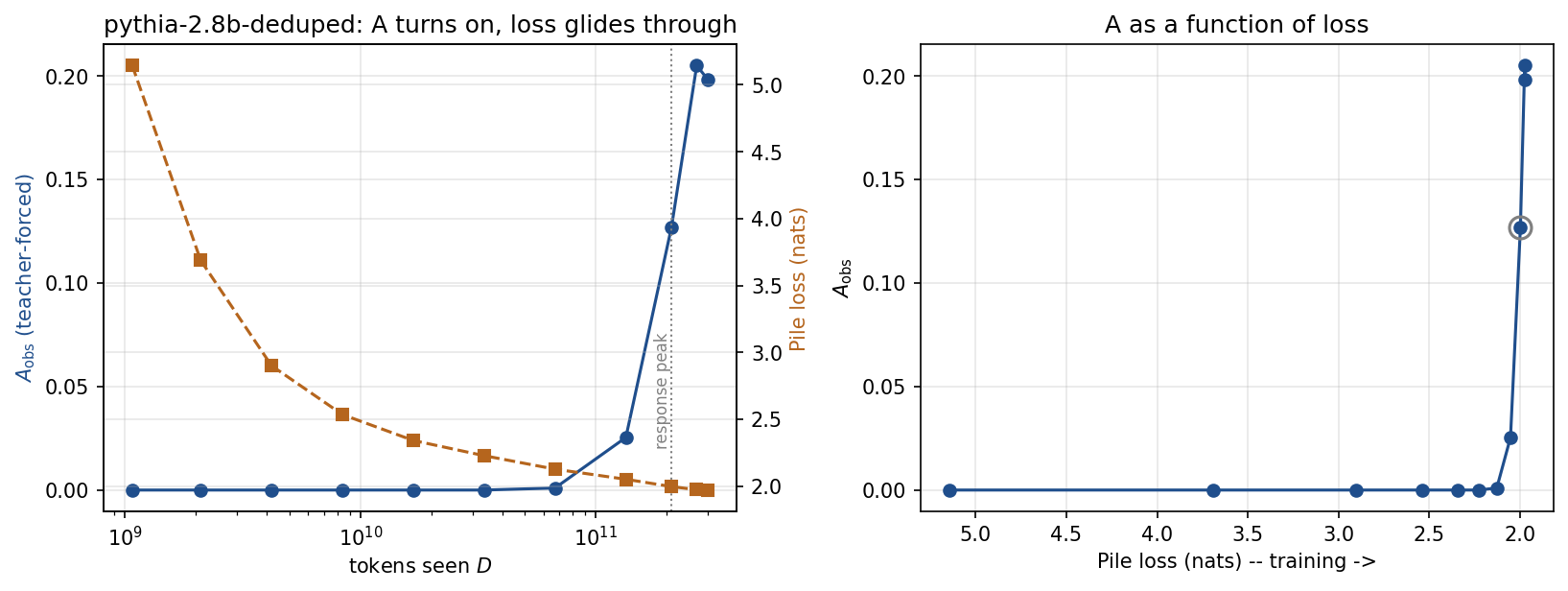The loss is the free energy, and it is a smooth, strictly monotone function of $D$; plotting $A$ against $L$ rather than against $\log D$ is a smooth invertible reparameterization of the control axis, and a smooth reparameterization can neither create a singularity nor change the order of one. Du et al.’s axis cannot manufacture a transition the $D$ axis lacks. Mapped explicitly — held-out Pile loss for the pythia-2.8b-deduped trajectory at the same checkpoints — the loss has no feature of its own where the accuracy turns on: the response peak at $D^* = 2.1\times10^{11}$ sits at $L \approx 2.0$ nats on a smooth, monotone stretch, the loss gliding by only about $0.15$ nats across the interval where $A$ climbs from $0.001$ to $0.205$. That shows the loss axis is a benign reparameterization here — not that smoothness rules out a transition, which, per the dictionary, it never could.

Worse for the rebuttal, the collapse onto a loss curve is predicted by composition: if per-token competence $p$ is a function of how well-trained the model is — same loss, same $p$ — then $A \approx p^{\ell}$ is automatically a function of loss alone, so the cross-size collapse Du et al. report is a consequence of the deflationary account, not evidence against it.

On this task the collapse is only partly visible, and worth showing as it is. Along the training axis the $d = 3$ accuracy of three sizes does lie on a common $A(L)$ curve, but only pythia-2.8b-deduped reaches low enough loss to climb it; pythia-1b and pythia-1.4b never clear $A \approx 0.01$ and so only pin the high-loss foot.

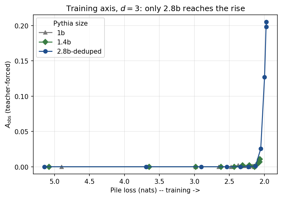
Accuracy versus Pile loss along training ($d = 3$), one curve per size, training running left as loss falls. Consistent with a single $A(L)$ curve, but only the largest size reaches low enough loss to enter the rise.

The parameter axis traces the same relation more fully: the eight final checkpoints, scored once each, fall on one rough $A(L)$ curve with the larger, lower-loss models carrying the turn-on — though the fit is only as clean as the suite, with pythia-6.9b sitting below trend, the documented anomaly in that model.

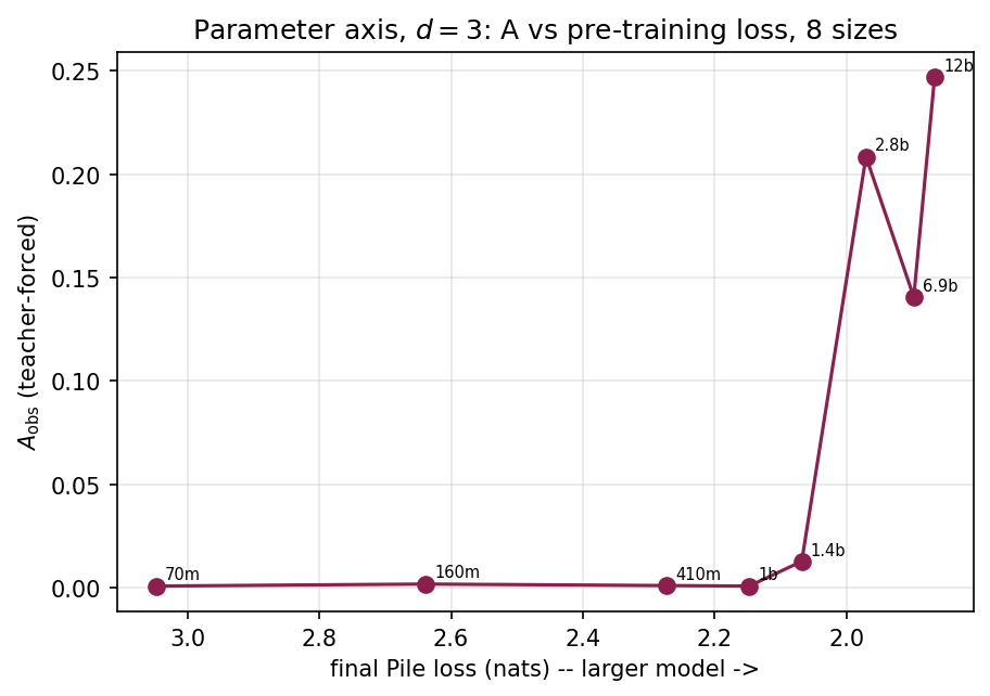
Teacher-forced accuracy versus final-checkpoint Pile loss across the eight sizes (70M–12B). Against pre-training loss rather than parameter count the sizes collapse onto one rough curve — what composition predicts, since $A \approx p^{\ell}$ inherits its loss-dependence from $p$.

The collapse is real but loose; what matters here is only that it is consistent with $A$ being a function of loss, as composition requires, and not a separate phenomenon demanding a transition. The two analyses then answer different questions. Du et al. rebut the metric-discontinuity claim — that sharpness is a hard-metric artifact that vanishes under a continuous metric; I grant the loss dependence, even in the continuous $p$, and ask about the order of the transition. By the dictionary that question is decided by the fluctuation susceptibility and the correlation length, on which the loss-collapse is silent: the connected correlation $\phi$ stays small, short-ranged, and non-diverging through $D^*$. A finite response peak on a flat, short-ranged correlation is a crossover dressed sharp by exact match — located consistently on every axis, collective on none.

Because the measurement runs along training in a single model, all of this speaks to the composition mechanism, not to emergence with parameter scale — that is Part I. The same caution applies there: $\phi(N)$ in Part I is the same $d = 3$ residual read across model sizes, so it carries the same length-pooling contamination and deserves the length-conditioned, digit-level treatment applied here before its small negative value is read as a correlation.

Reproducibility

Hardware, precision, and the evaluation pipeline are exactly as in Part I. The checkpoint sweep, the length-conditioned and digit-level error analyses, and the script regenerating every figure here are in scaling-experiments, with the executed notebook alongside.

---

Prose edited with the assistance of Claude (Anthropic), which also checked the numbers against the analysis artifacts and ran supplementary experiments. I ran the main experiments and vouch for every claim here.